

Describing your scanner: the geometry#
Every TIGRE operation takes three things: the data (an image or a set of projections), a geometry that describes the scanner, and the angles at which the projections were taken. This page explains the geometry fields, the coordinate system they live in, and how to describe less common scanners.
Coordinate system#
TIGRE uses a right-handed coordinate system centred on the origin, the point the source and detector rotate around.
At angle 0 the source sits on the positive x axis, at a distance
DSOfrom the origin, and the detector sits on the other side, at a distanceDSDfrom the source.The detector’s
uaxis (its columns) is parallel to y, and itsvaxis (its rows) is parallel to z.A positive angle rotates the source and detector around the z axis.
The image is centred on the origin unless you move it with
offOrigin.
To see your own geometry, plot it:
import numpy as np
import tigre

geo = tigre.geometry_default()
tigre.plot_geometry(geo, angle=-np.pi / 6)
geo = defaultGeometry();
plotgeometry(geo, -pi/6);
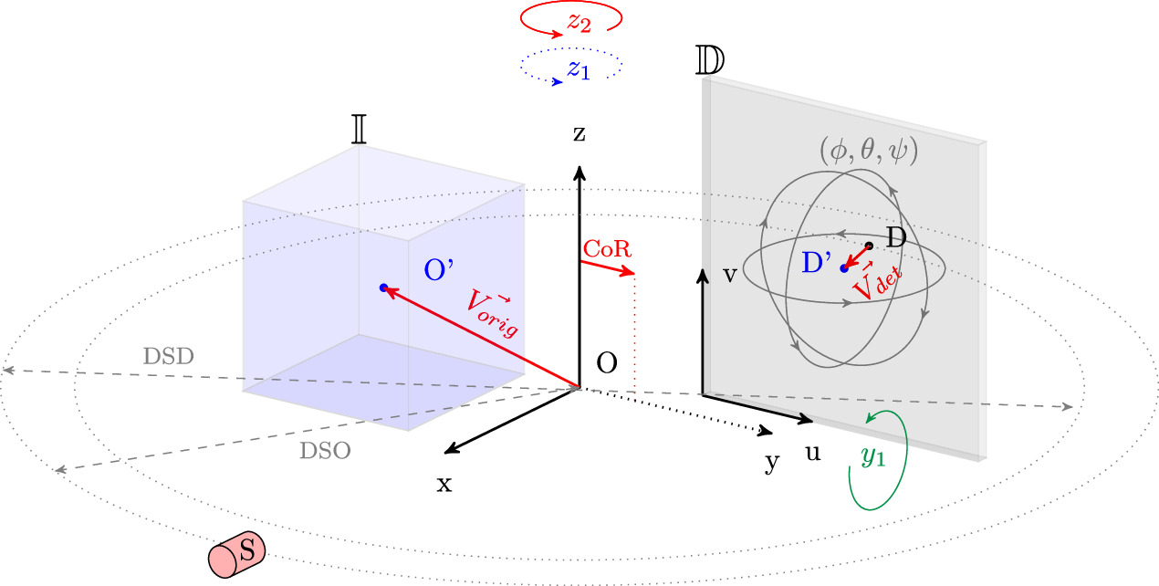
TIGRE’s geometry for one projection, with the names of the geo fields.
From Biguri et al. (2025), TIGRE v3,
figure 1 (CC BY 4.0). MATLAB’s
showGeoCBCTDiagram shows a similar diagram.#
The fields#
All distances are in millimetres (any unit works, as long as every field uses the same one) and all angles are in radians.
Field |
Size |
Meaning |
|---|---|---|
|
1, or one per angle |
Distance from the source to the detector. |
|
1, or one per angle |
Distance from the source to the origin. |
|
2 |
Number of detector pixels. |
|
2 |
Size of one detector pixel. |
|
2 |
Total size of the detector, |
|
3 |
Number of voxels in the image. |
|
3 |
Size of one voxel. |
|
3 |
Total size of the image, |
|
3, or 3 per angle |
Shift of the image centre from the origin. Optional, default 0. |
|
2, or 2 per angle |
Shift of the detector centre. Optional, default 0. |
|
3, or 3 per angle |
Detector rotation (roll, pitch, yaw). Optional, default 0. |
|
1, or one per angle |
Centre-of-rotation shift, along y. Optional, default 0. |
|
1 |
Sampling step of the |
|
text |
|
TIGRE checks that nVoxel * dVoxel equals sVoxel, and that
nDetector * dDetector equals sDetector, and raises an error if they don’t
match. Set all three of each group, as in the example below.
Python and MATLAB order the axes differently#
This is the most common source of confusion when moving code between the two languages.
MATLAB stores vectors in
(x, y, z)order for the image and(u, v)for the detector, and images are indexedimg(x, y, z).Python reverses them to match NumPy’s index order:
(z, y, x)for the image and(v, u)for the detector. Images are indexedimg[z, y, x]and projectionsproj[angle, v, u].
This applies to nVoxel, dVoxel, sVoxel, offOrigin, nDetector,
dDetector, sDetector and offDetector. rotDetector is the exception:
it is (roll, pitch, yaw) in both languages.
For example, moving the image 10 mm along the rotation axis is
geo.offOrigin = [0; 0; 10] in MATLAB and
geo.offOrigin = np.array([10, 0, 0]) in Python.
A complete example#
import numpy as np
import tigre

geo = tigre.geometry()
# Distances
geo.DSD = 1536                                  # source to detector (mm)
geo.DSO = 1000                                  # source to origin (mm)
# Detector, in (v, u) order
geo.nDetector = np.array([512, 512])            # pixels
geo.dDetector = np.array([0.8, 0.8])            # pixel size (mm)
geo.sDetector = geo.nDetector * geo.dDetector   # detector size (mm)
# Image, in (z, y, x) order
geo.nVoxel = np.array([256, 256, 256])          # voxels
geo.sVoxel = np.array([256, 256, 256])          # image size (mm)
geo.dVoxel = geo.sVoxel / geo.nVoxel            # voxel size (mm)
# Optional
geo.offOrigin = np.array([0, 0, 0])             # image offset (mm)
geo.offDetector = np.array([0, 0])              # detector offset (mm)
geo.accuracy = 0.5                              # interpolated projector step (voxels)
geo.mode = "cone"

angles = np.linspace(0, 2 * np.pi, 360, endpoint=False)
print(geo)
% Distances
geo.DSD = 1536;                             % source to detector (mm)
geo.DSO = 1000;                             % source to origin (mm)
% Detector, in (u, v) order
geo.nDetector = [512; 512];                 % pixels
geo.dDetector = [0.8; 0.8];                 % pixel size (mm)
geo.sDetector = geo.nDetector .* geo.dDetector;
% Image, in (x, y, z) order
geo.nVoxel = [256; 256; 256];               % voxels
geo.sVoxel = [256; 256; 256];               % image size (mm)
geo.dVoxel = geo.sVoxel ./ geo.nVoxel;      % voxel size (mm)
% Optional
geo.offOrigin = [0; 0; 0];                  % image offset (mm)
geo.offDetector = [0; 0];                   % detector offset (mm)
geo.accuracy = 0.5;                         % interpolated projector step (voxels)
geo.mode = 'cone';

angles = linspace(0, 2*pi, 360);
angles(end) = [];
If you are just experimenting, the default geometries save typing:
tigre.geometry_default(high_resolution=False) in Python (a 64³ image) or
defaultGeometry('nVoxel', [64; 64; 64]) in MATLAB.
Angles#
angles is usually a vector of N rotation angles in radians, one per
projection. TIGRE does not need them to be equally spaced, sorted or to
cover a full circle.
You can also give an N×3 array (3×N in MATLAB). Each row is then a set of ZYZ Euler angles, which describes source and detector trajectories that are not a circle around z. See the arbitrary-axis demo (Python, MATLAB). FDK does not support these geometries; use an iterative algorithm.
Fields that change per projection#
DSD, DSO, offOrigin, offDetector, rotDetector and COR can be
given once, or once per angle. A per-angle value lets you describe
geometries that are not a plain circular scan.
Helical scans. Move the image along the rotation axis at each angle with
offOrigin. In Python that is column 0, geo.offOrigin[:, 0]; in MATLAB it
is row 3, geo.offOrigin(3, :). See demo 13
(Python,
MATLAB).
Detector offsets. A detector shifted sideways, for example to widen the
field of view with a half-fan scan, is described with offDetector. See
demo 14 (Python,
MATLAB).
Detector rotation. Small misalignments of the detector are described with
rotDetector. The first value (roll) rotates the detector within its own
plane, which is usually the only one that needs correcting in practice. See
demo 17 (Python,
MATLAB).
Centre of rotation. If the rotation axis does not project onto the centre
of the detector, set COR. TIGRE can estimate it from the data with
tigre.computeCOR (Python) or computeCOR (MATLAB).
Fixed detectors and moving sources. Python has helpers that build
per-angle geometries for these cases: tigre.staticDetectorGeo,
tigre.staticDetLinearSourceGeo and tigre.ArbitrarySourceDetMoveGeo.
Other scanner types#
Parallel beam. Set geo.mode = "parallel". All rays are then parallel;
DSD and DSO only set where each ray starts and ends, so keep both ends
outside the image. In Python,
tigre.geometry(mode="parallel", nVoxel=np.array([nz, ny, nx])) builds a
parallel geometry with one-millimetre voxels and pixels. See demo 15.
2D tomography. TIGRE is a 3D code, so a 2D problem is a 3D problem one
voxel thick: set the image to 1 slice and the detector to 1 row, and make the
detector pixel height equal to the voxel height. In Python that means
nVoxel = [1, ny, nx] and nDetector = [1, nu]. See demo 16.
Digital breast tomosynthesis. A limited-angle cone-beam scan; see demo 19.
Curved detectors. TIGRE’s projectors assume a flat detector. Resample
curved-detector data onto a flat detector first with flatten_detector
(in Python, from tigre.utilities.curved_detector import flatten_detector),
then reconstruct as usual. See the curved-detector demo (d24 in Python,
d024 in MATLAB).
Checking your geometry#
Most reconstruction problems are geometry problems. Before tuning an algorithm:
Plot the geometry and check that the image sits inside the cone of rays.
Reconstruct with FDK (or FBP for parallel beam). Blurred or doubled edges usually mean a wrong
COR, a wrongoffDetectoror the wrong sign of the angles.Forward-project your reconstruction with
Axand compare it with your measured projections. They should line up.