

Note
Go to the end to download the full example code.
Plot images and projections#
All the options of plotimg and plotproj.
Source: Python/demos/d05_plottingFunctions.py · MATLAB/Demos/d05_plottingFunctions.m
MATLAB version of this demo
%% Demo 5: How to use plotting functions
%
% This demo will demonstrate the options for plotting projection and images
% on TIGRE. The functions have been in previous demos, but in here an
% exhaustive explanation and usage of them is given.
%
%
%--------------------------------------------------------------------------
%--------------------------------------------------------------------------
% This file is part of the TIGRE Toolbox
%
% Copyright (c) 2015, University of Bath and
%                     CERN-European Organization for Nuclear Research
%                     All rights reserved.
%
% License:            Open Source under BSD.
%                     See the full license at
%                     https://github.com/CERN/TIGRE/blob/master/LICENSE
%
% Contact:            tigre.toolbox@gmail.com
% Codes:              https://github.com/CERN/TIGRE/
% Coded by:           Ander Biguri
%--------------------------------------------------------------------------
%% Initialize

clear;
close all;
%% Define Geometry
geo=defaultGeometry('nVoxel',[128;128;128]);

%% Load data and generate projections
% see previous demo for explanation
angles=linspace(0,2*pi,100);
head=headPhantom(geo.nVoxel);
projections=Ax(head,geo,angles,'interpolated');
noise_projections=addCTnoise(projections);
%% Reconstruct image using OS-SART and FDK
imgFDK=FDK(noise_projections,geo,angles);
imgOSSART=OS_SART(noise_projections,geo,angles,50);


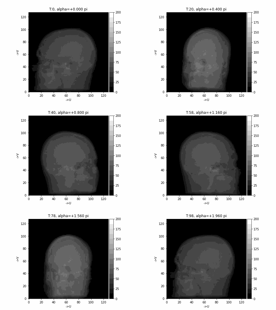
%% Lets use PlotProj
%
% plotProj plots the projection data measure on the detector on each angle.
%
% exhaustive list of possible parameters:

% 'Step' : Defines the step size for skippin projections when plotting,
% usefull when there are a big amount of projections. Default is 1
step=2;

% 'Colormap': Defines the colormap used to plot. Default is 'gray'. any
% MATLAB colromap can be used, also any user created Nx3 colorpam can be
% used. Additionally, TIGRE includes perceptually uniform colormaps, where
% ?color == ?data. The perceptuall uniform options are the default 'gray',
%  abd 'magma', 'viridis', 'inferno' and 'plasma'

colormap=hsv(10);
colormap='gray';
colormap='viridis';
colormap='plasma';
colormap='gray';

% 'Clims': Defines the data limits for the color, usefull when one wants to
% see some specific range. The default uses the minimum and maximum of the
% data.

clims=[0 200];

% 'Savegif': allows to save the plotted figure as an animated gif,
% specified by the given filename.

giffilename='demo5projections.gif';

% 'Slice': allows to plot a single projection .Will overwrite the behavior
% of 'Step'
slice=5;

% Lets try out.
plotProj(noise_projections,angles,'Step',step,'Colormap',colormap,'CLims',clims,'Savegif',giffilename); % not using 'Step'

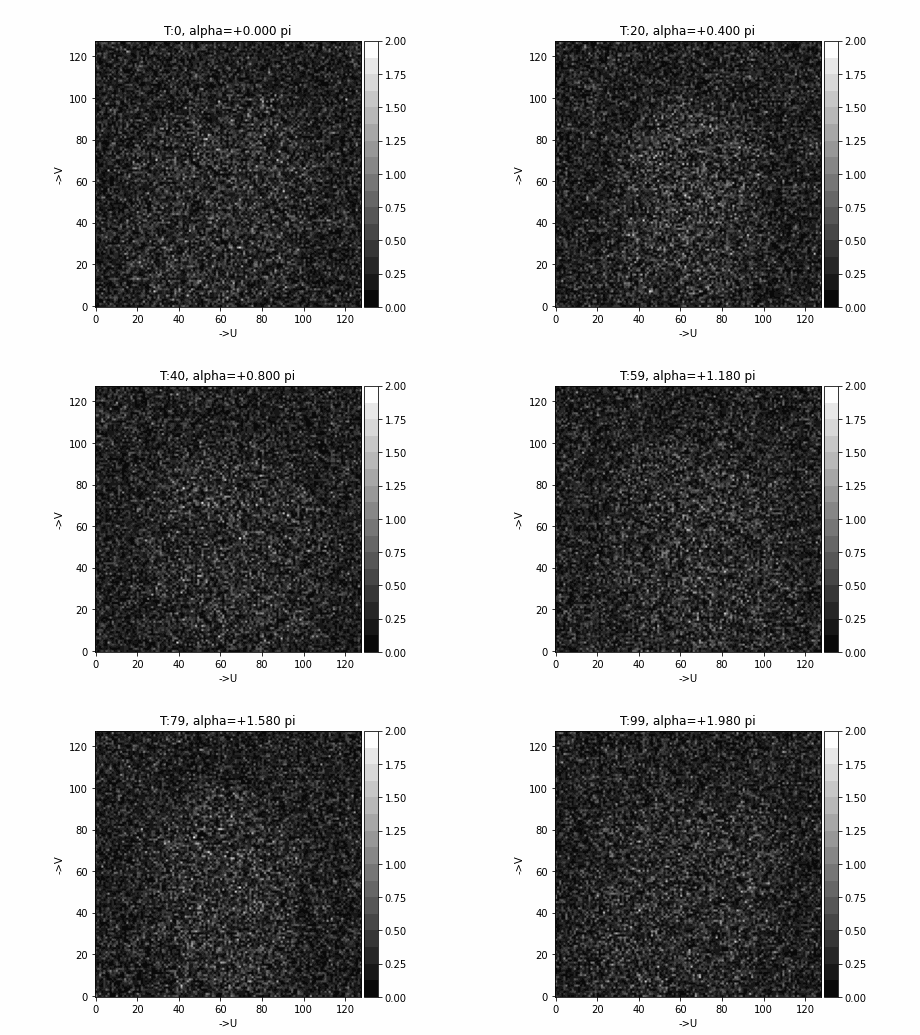
% Remember you can also plot errors, for example the added noise by:

noise=abs(noise_projections-projections); %abs is what we are interested in plotting
plotProj(noise,angles,'CLims',[0,2]);


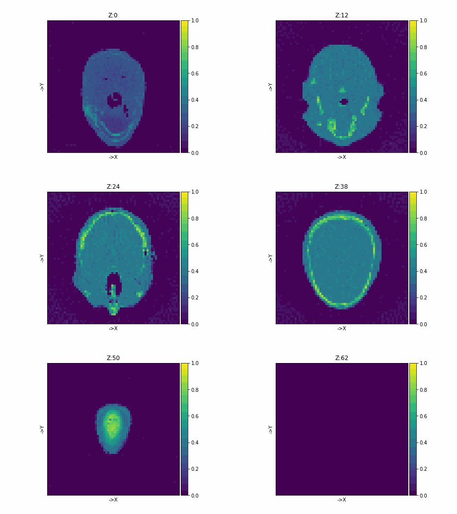
%% What about plotting the Image? plotImg()
%
% plotImg plots the image slice by slice.
%
% List of optional parameters:


% 'Dim': specifies the dimension for plotting.
%    Dim can be 'X','Y','Z' or 1, 2 ,3 (being the same)
%
dimension='Z'; % or 'z' or 3

% 'Step': step size of the plotting. Useful when images are big or one just
% wants an overview of the result

step=2;
% 'Colormap': Defines the colormap used to plot. Default is 'gray'. any
% MATLAB colromap can be used, also any user created Nx3 colorpam can be
% used. Additionally, TIGRE includes perceptually uniform colormaps, where
% ?color == ?data. The perceptuall yuniform options are the default 'gray',
% 'magma', 'viridis', 'inferno' and 'plasma'

colormap=hsv(20);
colormap='magma';
colormap='viridis';
colormap='gray';

% 'Clims': Defines the data limits for the color, usefull when one wants to
% see some specific range. The default computes the 5% and 95% percentiles
% of the data and uses that as limit.

clims=[0 01];

% 'Savegif': allows to save the plotted figure as an animated gif,
% specified by the given filename.

giffilename='demo5image.gif';

% 'Slice': allows to plot a single slice .Will overwrite the behavior
% of 'Step'
slice=64;

% Lets go for it

plotImg(imgFDK,'Dim',dimension,'Step',step,'CLims',clims,'Colormap',colormap,'Savegif',giffilename);

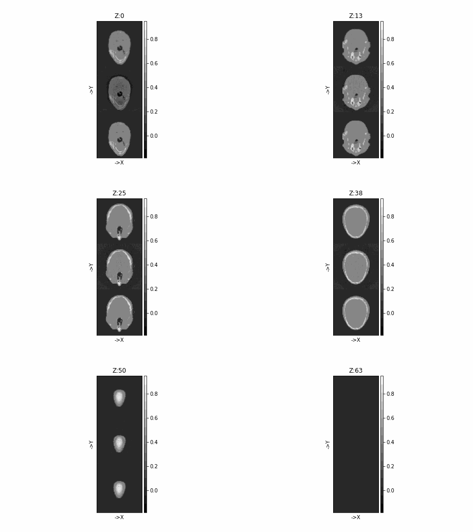
% Remember: You can always plot more than 1 image together!
plotImg([head imgFDK imgOSSART],'Dim','z')
% Or even the errors!
plotImg([abs(head-imgFDK) abs(head-imgOSSART)],'Dim',3);
Initialize#
import tigre
import numpy as np
from tigre.utilities import sample_loader
from tigre.utilities import CTnoise
import tigre.algorithms as algs
Geometry#
geo = tigre.geometry_default(high_resolution=False)
Load data and generate projections#
# define angles
angles = np.linspace(0, 2 * np.pi, 100, endpoint=False)
# Load thorax phantom data
head = sample_loader.load_head_phantom(geo.nVoxel)
# generate projections
projections = tigre.Ax(head, geo, angles)
# add noise
noise_projections = CTnoise.add(projections, Poisson=1e5, Gaussian=np.array([0, 10]))
Reconstruct image using OS-SART and FDK#
# FDK
imgFDK = algs.fdk(noise_projections, geo, angles)
niter = 50
imgOSSART = algs.ossart(noise_projections, geo, angles, 50)
OSSART algorithm in progress.
Estimated time until completion : 00:00:03
Algorithm will finish at        : 16:48:06
Lets use PlotProj#
#
# plotProj plots the projection data measure on the detector on each angle.
#
# exhaustive list of possible parameters:

# 'Step' : Defines the step size for skippin projections when plotting,
# usefull when there are a big amount of projections. Default is 1
step = 2

# 'Colormap': Defines the colormap used to plot. Default is 'gray'.

colormap = "viridis"
colormap = "plasma"
colormap = "gray"

# 'Clims': Defines the data limits for the color, usefull when one wants to
# see some specific range. The default uses the minimum and maximum of the
# data.

clims = [0, 200]

# 'Savegif': allows to save the plotted figure as an animated gif,
# specified by the given filename.

giffilename = "demo5projections.gif"

# 'Slice': allows to plot a single projection .Will overwrite the behavior
# of 'Step'
slice = 5

# Lets try out.
tigre.plotproj(
    noise_projections, angles, step=step, colormap=colormap, clims=clims, savegif=giffilename
)  # not using 'Step'

# Remember you can also plot errors, for example the added noise by:

noise = np.abs(noise_projections - projections)  # abs is what we are interested in plotting
tigre.plotproj(noise, angles, clims=[0, 2])
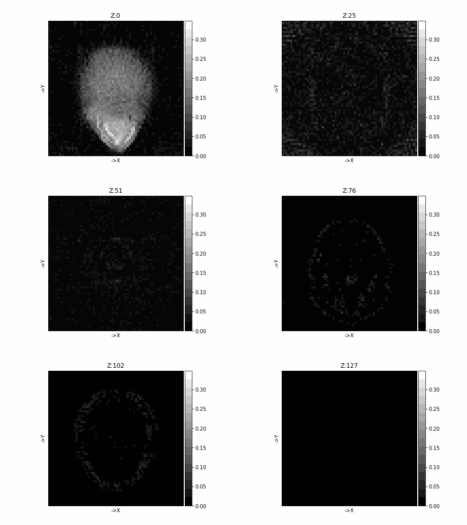
PlotImg#
# plotImg plots the image slice by slice.
#
# List of optional parameters:

# 'Dim': specifies the dimension for plotting.
#    Dim can be 'X','Y','Z'
#
dimension = "Z"

# 'Step': step size of the plotting. Useful when images are big or one just
# wants an overview of the result

step = 2
# 'Colormap': Defines the colormap used to plot. Default is 'gray'.

colormap = "plasma"
colormap = "magma"
colormap = "gray"
colormap = "viridis"

# 'Clims': Defines the data limits for the color, usefull when one wants to
# see some specific range. The default computes the 5% and 95% percentiles
# of the data and uses that as limit.

clims = [0, 1]

# 'Savegif': allows to save the plotted figure as an animated gif,
# specified by the given filename.

giffilename = "demo5image.gif"

# 'Slice': allows to plot a single slice .Will overwrite the behavior
# of 'Step'
slice = 64

# Lets go for it

tigre.plotimg(imgFDK, dim=dimension, step=step, clims=clims, colormap=colormap, savegif=giffilename)

# Remember: You can always plot more than 1 image together!
tigre.plotimg(np.concatenate([head, imgFDK, imgOSSART], axis=1), dim="z")
# Or even the errors!
tigre.plotImg(np.concatenate([np.abs(head - imgFDK), np.abs(head - imgOSSART)]), dim="z")
Total running time of the script: (0 minutes 45.074 seconds)