

Note
Go to the end to download the full example code.
Measure image quality#
Compute error and similarity measures against a reference image, also during the iterations of an algorithm.
Source: Python/demos/d10_MeasureQuality.py · MATLAB/Demos/d10_QualityMeasurements.m
MATLAB version of this demo
%% Demo 10: How to use Image quality measures
%
% This demo demonstrate how to compute all the image quality measures
% by calling the "Measure_Quality.m" function with detailed description.
%
%
%--------------------------------------------------------------------------
%--------------------------------------------------------------------------
% This file is part of the TIGRE Toolbox
%
% Copyright (c) 2015, University of Bath and
%                     CERN-European Organization for Nuclear Research
%                     All rights reserved.
%
% License:            Open Source under BSD.
%                     See the full license at
%                     https://github.com/CERN/TIGRE/blob/master/LICENSE
%
% Contact:            tigre.toolbox@gmail.com
% Codes:              https://github.com/CERN/TIGRE/
% Coded by:           Manasavee Lohvithee
%--------------------------------------------------------------------------
%% Initialize

clear;
close all;
%% Define Geometry
%
geo=defaultGeometry('nVoxel',[128;128;128]);

%% Load data and generate projections
% see previous demo for explanation
angles=linspace(0,2*pi,100);
head=headPhantom(geo.nVoxel);
projections=Ax(head,geo,angles,'interpolated');
noise_projections=addCTnoise(projections);

%% "Measure_Quality.m" function
% There are three inputs to the function
%
% "res_prev"  is a set of real phantom image or reconstructed image from
%             the previous iteration (in case you want to compare the image
%             quality measure after each iteration)
%
% "res"       is a set of final reconstructed image or reconstructed image
%             from the current iteration (in case you want to compare the image
%             quality measure after each iteration)
%
% "QualMeasOpts"  contains a cell array of desired quality measurement names.
%                 Example: {'CC','RMSE','MSSIM','UQI'}. At the moment,
%                 there are 4 image quality measures as following:
%
%           'RMSE' : The square root of the mean of the squared differences
%                    of pixel intensities of two images.
%
%                    Taken from "A rigid motion correction method for helical
%                    computed tomography (CT)"
%                    (doi:10.1088/0031-9155/60/5/2047)
%
%           'CC'   : The Pearson correlation coefficient which measures the
%                    linear dependence between two images.
%
%                    Taken from "A rigid motion correction method for helical
%                    computed tomography (CT)"
%                    (doi:10.1088/0031-9155/60/5/2047)
%
%           'MSSIM': The mean structural similarity index, a measure of the
%                    similarity of two images in terms of luminance,
%                    contrast and structure that is designed to provide a
%                    good approximation of perceptual image quality.
%
%                    Taken from "A rigid motion correction method for helical
%                    computed tomography (CT)"
%                    (doi:10.1088/0031-9155/60/5/2047)
%
%           'UQI' : The universal quality index to evaluate the degree of
%                   similarity between the reconstructed and phantom images
%                   for chosen ROIs. Its value ranges from zero to one.
%                   A UQI value closer to one suggests better similarity to true image.
%
%                   Taken from "Few-view cone-beam CT reconstruction with
%                   deformed prior image" (doi: 10.1118/1.4901265)
%
%
%
%

%% Define a cell array of image quality measures
qualmeas={'RMSE','CC','MSSIM','UQI'};

blcks=22;

%% Reconstruct image using SIRT, SART and OS-SART

[imgSIRT,errL2SIRT,qualitySIRT]=SIRT(noise_projections,geo,angles,30,...
                            'QualMeas',qualmeas);
[imgSART,errL2SART,qualitySART]=SART(noise_projections,geo,angles,30,...
                            'QualMeas',qualmeas);
[imgOSSART,errL2OSSART,qualityOSSART]=OS_SART(noise_projections,geo,angles,30,...
                            'QualMeas',qualmeas,'BlockSize',blcks);


%% Plot the changes of image quality measures over iterations

%%RMSE plot (and the other requested metrics)
% Each algorithm may stop at a different iteration. Plot its own history
% directly, preserving legitimate zeros and avoiding assumptions about length.
histories={qualitySIRT,qualitySART,qualityOSSART};
algorithmNames={'SIRT','SART','OS-SART'};
metricNames={'RMSE','CC','MSSIM','UQI'};
for metric=1:numel(metricNames)
    figure;
    hold on;
    for algorithm=1:numel(histories)
        values=histories{algorithm}(metric,:);
        plot(1:numel(values),values,'DisplayName',algorithmNames{algorithm});
    end
    title(['Evolution of ' metricNames{metric} ' per iteration']);
    xlabel('Iteration');
    ylabel(metricNames{metric});
    legend('show');
end

%% Compute the parameters for the target image
% Knowing change of the parameters per iteration can be interesting, but
% the main use of them would be to compare a reconstructed image to a given
% known target image.

disp('UQI for SART,   SIRT,   OS-SART')
disp(['       ',num2str(UQI(head,imgSART)),' ', num2str(UQI(head,imgSIRT)),' ' ,num2str(UQI(head,imgOSSART))])
disp('RMSE for SART,   SIRT,   OS-SART')
disp(['       ',num2str(RMSE(head,imgSART)),' ', num2str(RMSE(head,imgSIRT)),' ' ,num2str(RMSE(head,imgOSSART))])
Initialize#
import tigre
import numpy as np
from tigre.utilities import sample_loader
from tigre.utilities import CTnoise
import tigre.algorithms as algs
from matplotlib import pyplot as plt
from tigre.utilities.Measure_Quality import Measure_Quality as MQ
Geometry#
geo = tigre.geometry_default(high_resolution=False)
Load data and generate projections#
# define angles
angles = np.linspace(0, 2 * np.pi, 100, endpoint=False)
# Load thorax phantom data
head = sample_loader.load_head_phantom(geo.nVoxel)
# generate projections
projections = tigre.Ax(head, geo, angles)
# add noise
noise_projections = CTnoise.add(projections, Poisson=1e5, Gaussian=np.array([0, 10]))
Image quality measurement#
# There are three inputs to the function

#
#           'RMSE' : The square root of the mean of the squared differences
#                    of pixel intensities of two images.
#
#                    Taken from "A rigid motion correction method for helical
#                    computed tomography (CT)"
#                    (doi:10.1088/0031-9155/60/5/2047)
#           'nRMSE': The square root of the mean of the squared differences
#                    of pixel intensities of two images, normalized
#
#           'CC'   : The Pearson correlation coefficient which measures the
#                    linear dependence between two images.
#
#                    Taken from "A rigid motion correction method for helical
#                    computed tomography (CT)"
#                    (doi:10.1088/0031-9155/60/5/2047)
#
#           'MSSIM': The mean structural similarity index, a measure of the
#                    similarity of two images in terms of luminance,
#                    contrast and structure that is designed to provide a
#                    good approximation of perceptual image quality.
#
#                    Taken from "A rigid motion correction method for helical
#                    computed tomography (CT)"
#                    (doi:10.1088/0031-9155/60/5/2047)
#
#           'UQI' : The universal quality index to evaluate the degree of
#                   similarity between the reconstructed and phantom images
#                   for chosen ROIs. Its value ranges from zero to one.
#                   A UQI value closer to one suggests better similarity to true image.
#
#                   Taken from "Few-view cone-beam CT reconstruction with
#                   deformed prior image" (doi: 10.1118/1.4901265)
#
#
#
#

## Define a cell array of image quality measures
qualmeas = ["RMSE", "CC", "MSSIM", "UQI"]
Reconstruct image using SIRT, SART and OS-SART#
# =========================================================================
imgSIRT, qualitySIRT = algs.sirt(noise_projections, geo, angles, 20, Quameasopts=qualmeas)
imgSART, qualitySART = algs.sart(noise_projections, geo, angles, 20, Quameasopts=qualmeas)
imgOSSART, qualityOSSART = algs.ossart(noise_projections, geo, angles, 20, Quameasopts=qualmeas)
SIRT algorithm in progress.
C:\Users\ander\anaconda3\envs\tigre\Lib\site-packages\numpy\lib\_function_base_impl.py:3023: RuntimeWarning: invalid value encountered in divide
  c /= stddev[:, None]
C:\Users\ander\anaconda3\envs\tigre\Lib\site-packages\numpy\lib\_function_base_impl.py:3024: RuntimeWarning: invalid value encountered in divide
  c /= stddev[None, :]
Estimated time until completion : 00:00:00
Algorithm will finish at        : 16:48:48
SART algorithm in progress.
Estimated time until completion : 00:00:12
Algorithm will finish at        : 16:49:02
OSSART algorithm in progress.
Estimated time until completion : 00:00:01
Algorithm will finish at        : 16:49:02
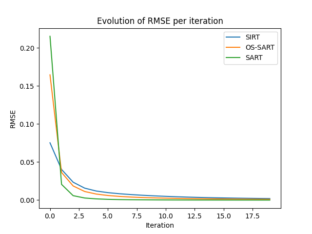
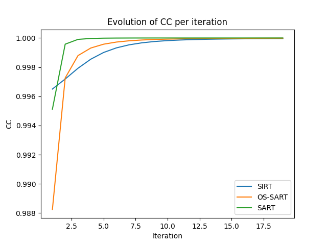
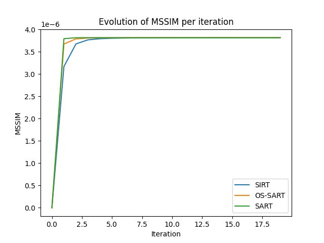
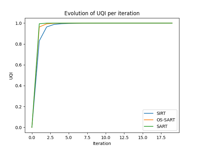
Plot the changes of image quality measures over iterations, i.e. how much each iteration looks like the previous iteration.#
# (without the original image one can not compute the absolute image quality, of course)

##RMSE plot
plt.figure()
plt.plot(np.vstack((qualitySIRT[0, :], qualityOSSART[0, :], qualitySART[0, :])).T)
plt.title("Evolution of RMSE per iteration")
plt.xlabel("Iteration")
plt.ylabel("RMSE")
plt.gca().legend(("SIRT", "OS-SART", "SART"))

##CC plot
plt.figure()
plt.plot(np.vstack((qualitySIRT[1, :], qualityOSSART[1, :], qualitySART[1, :])).T)
plt.title("Evolution of CC per iteration")
plt.xlabel("Iteration")
plt.ylabel("CC")
plt.gca().legend(("SIRT", "OS-SART", "SART"))

##MSSIM plot
plt.figure()
plt.plot(np.vstack((qualitySIRT[2, :], qualityOSSART[2, :], qualitySART[2, :])).T)
plt.title("Evolution of MSSIM per iteration")
plt.xlabel("Iteration")
plt.ylabel("MSSIM")
plt.gca().legend(("SIRT", "OS-SART", "SART"))

##UQI plot
plt.figure()
plt.plot(np.vstack((qualitySIRT[3, :], qualityOSSART[3, :], qualitySART[3, :])).T)
plt.title("Evolution of UQI per iteration")
plt.xlabel("Iteration")
plt.ylabel("UQI")
plt.gca().legend(("SIRT", "OS-SART", "SART"))

plt.show()
Compute the parameters for the target image#
# Knowing change of the parameters per iteration can be interesting, but
# The main use of them would be to compare a reconstructed image to a given
# known target image.

sart_uqi = MQ(head, imgSART, ["UQI"])
sirt_uqi = MQ(head, imgSIRT, ["UQI"])
ossart_uqi = MQ(head, imgOSSART, ["UQI"])

print("UQI for SART,   SIRT,   OS-SART")
print("       " + str(sart_uqi) + " " + str(sirt_uqi) + " " + str(ossart_uqi))

sart_rmse = MQ(head, imgSART, ["RMSE"])
sirt_rmse = MQ(head, imgSIRT, ["RMSE"])
ossart_rmse = MQ(head, imgOSSART, ["RMSE"])

print("RMSE for SART,   SIRT,   OS-SART")
print("       " + str(sart_rmse) + " " + str(sirt_rmse) + " " + str(ossart_rmse))
UQI for SART,   SIRT,   OS-SART
       0.9996299654256502 0.9481986239371448 0.9930949515753248
RMSE for SART,   SIRT,   OS-SART
       0.005299152075107854 0.05864690912342974 0.022644113658784406
Total running time of the script: (0 minutes 15.757 seconds)