

Note
Go to the end to download the full example code.
Projectors and backprojectors#
Siddon and interpolated projection, FDK-weighted and matched backprojection. See Projection and backprojection.
Source: Python/demos/d12_ProjectionOperations.py · MATLAB/Demos/d12_ProjectionOperators.m
MATLAB version of this demo
%% DEMO 12: Understanding different Forward projections
%
%
%  In this more advanced demo, an explanation of the difference between the
%  forward projections will be given.
%
%  While there are 2 backprojectors, these are less different, they just
%  have different weights. One of the has a FDK weightt and the other on has
%  a weight that makes it mathematically very close to the transpose of
%  matrix A.
%
%
%--------------------------------------------------------------------------
%--------------------------------------------------------------------------
% This file is part of the TIGRE Toolbox
%
% Copyright (c) 2015, University of Bath and
%                     CERN-European Organization for Nuclear Research
%                     All rights reserved.
%
% License:            Open Source under BSD.
%                     See the full license at
%                     https://github.com/CERN/TIGRE/blob/master/LICENSE
%
% Contact:            tigre.toolbox@gmail.com
% Codes:              https://github.com/CERN/TIGRE/
% Coded by:           Ander Biguri
%--------------------------------------------------------------------------
%% Initialize
clear;
close all;

%% Define Geometry
%
geo=defaultGeometry('nVoxel',[128;128;128]);


%% This parameter is key for the accuracy of the interpolated FWD projection.
geo.accuracy=0.5;                           % Accuracy of FWD proj          (vx/sample)

%% Description
% The difference between them is that `Siddon` will compute the
% intersection of a ray crossing each voxel, and the `interpolated` will
% sample the voxels at a given sample rate.

%% Main difference

shepp=sheppLogan3D(geo.nVoxel);
tic
projInterp=Ax(shepp,geo,0,'interpolated');
interptime=toc;
tic
projray   =Ax(shepp,geo,0,'Siddon');
raytime=toc;
% It is relatively clear that discretization artifacts appear with the
% ray-voxel approach
plotProj([projInterp projray abs(projInterp-projray)],0);
% But also the ray voxel approach is faster (more obvious at bigger sizes)
disp(['Time interpolated: ' num2str(interptime)]);
disp(['Time Siddon      : ' num2str(raytime)]);
disp('Press enter to continue')
pause
%% We can play with the accuracy value

% With small voxel the errors are more obvious
geo.nVoxel=[32;32;32];                      % number of voxels              (vx)
geo.sVoxel=[256;256;256];                   % total size of the image       (mm)
geo.dVoxel=geo.sVoxel./geo.nVoxel;          % size of each voxel            (mm)
shepp=sheppLogan3D(geo.nVoxel);

geo.accuracy=3;
projInterp3=Ax(shepp,geo,0,'interpolated');
geo.accuracy=1;
projInterp1=Ax(shepp,geo,0,'interpolated');
geo.accuracy=0.5;
projInterp05=Ax(shepp,geo,0,'interpolated');
geo.accuracy=0.2;
projInterp02=Ax(shepp,geo,0,'interpolated');
geo.accuracy=0.05;
projInterp3005=Ax(shepp,geo,0,'interpolated');
geo.accuracy=0.01;
projInterp3001=Ax(shepp,geo,0,'interpolated');

% the error varies, at big accuracy values because interpolated option
% samples too few, but at small values because ray-voxel creates
% discretization artifacts
% ---------------------------------------------------------------------

% However It looks like while there is a big difference between the biggest
% and smallers, from accuracy from 1 to 0.01 there is no much change
plotProj([abs(projInterp02-projray) abs(projInterp3005-projray) abs(projInterp3001-projray);...
          abs(projInterp3-projray) abs(projInterp1-projray) abs(projInterp05-projray)],0,'CLims',[0 20]);

disp('Press enter to continue')
pause
% lets test the all accuracies against the smallest geo.accuracy value
% ---------------------------------------------------------------------
%
% Observe the colorbars. Note that the maximum value of the projection is
% around 60~, meaning a value of error of 14, is very relevant, while a
% value of error of 0.1 is less.
plotProj(abs(projInterp3-projInterp3001),0);
title('geo.accuracy=3')

plotProj(abs(projInterp1-projInterp3001),0);
title('geo.accuracy=1')

plotProj(abs(projInterp05-projInterp3001),0);
title('geo.accuracy=0.5')

plotProj(abs(projInterp02-projInterp3001),0);
title('geo.accuracy=0.2')

plotProj(abs(projInterp3005-projInterp3001),0);
title('geo.accuracy=0.05')

% From these plots we can conclude that  a value of 1 or less of
% geo.accuracy i srasonable. The smaller the better, but eventually the
% error will be so small that the imporvement is unperceptible. we
% recommend something in the range [0.1-0.5]
Initialize#
import tigre
import numpy as np
from tigre.utilities import sample_loader
import time
Geometry#
geo = tigre.geometry_default(high_resolution=False)
This parameter is key for the accuracy of the interpolated FWD projection.#
geo.accuracy = 0.5
# Accuracy of FWD proj          (vx/sample)

# lets do just one angles

angles = np.array([0])
Description#
# The difference between them is that `Siddon` will compute the
# intersection of a ray crossing each voxel, and the `interpolated` will
# sample the voxels at a given sample rate.
Main difference#
head = sample_loader.load_head_phantom(geo.nVoxel)
start_time = time.time()
projInterp = tigre.Ax(head, geo, angles, "interpolated")
interptime = time.time() - start_time

start_time = time.time()
projray = tigre.Ax(head, geo, angles, "Siddon")
raytime = time.time() - start_time
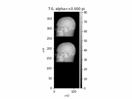
# It is relatively clear that discretization artifacts appear with the
# ray-voxel approach (middle one)
tigre.plotproj(np.concatenate([np.abs(projInterp - projray), projray, projInterp], axis=1), angles)
# But also the ray voxel approach is faster (more obvious at bigger sizes)
print("Time interpolated: " + str(interptime))
print("Time Siddon      : " + str(raytime))
Time interpolated: 0.008150577545166016
Time Siddon      : 0.004004478454589844
With small voxel the errors are more obvious#
geo.nVoxel = np.array([32, 32, 32])  # number of voxels              (vx)
geo.sVoxel = np.array([256, 256, 256])  # total size of the image       (mm)
geo.dVoxel = geo.sVoxel / geo.nVoxel  # size of each voxel            (mm)
head = sample_loader.load_head_phantom(geo.nVoxel)

geo.accuracy = 3
projInterp3 = tigre.Ax(head, geo, angles, "interpolated")
geo.accuracy = 1
projInterp1 = tigre.Ax(head, geo, angles, "interpolated")
geo.accuracy = 0.5
projInterp05 = tigre.Ax(head, geo, angles, "interpolated")
geo.accuracy = 0.2
projInterp02 = tigre.Ax(head, geo, angles, "interpolated")
geo.accuracy = 0.05
projInterp3005 = tigre.Ax(head, geo, angles, "interpolated")
geo.accuracy = 0.01
projInterp3001 = tigre.Ax(head, geo, angles, "interpolated")

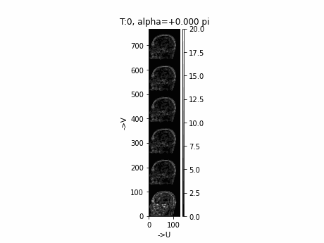
# the error varies, at big accuracy values because interpolated option
# samples too few, but at small values because ray-voxel creates
# discretization artifacts
# ---------------------------------------------------------------------

# However It looks like while there is a big difference between the biggest
# and smallers, from accuracy from 1 to 0.01 there is no much change
tigre.plotproj(
    np.concatenate(
        [
            np.abs(projInterp3 - projray),
            np.abs(projInterp1 - projray),
            np.abs(projInterp05 - projray),
            np.abs(projInterp02 - projray),
            np.abs(projInterp3005 - projray),
            np.abs(projInterp3001 - projray),
        ],
        axis=1,
    ),
    angles,
    clims=[0, 20],
)

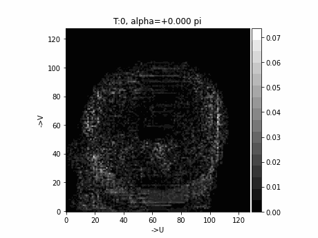
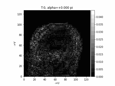
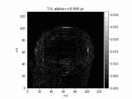
# lets test the all accuracies against the smallest geo.accuracy value
# ---------------------------------------------------------------------
#
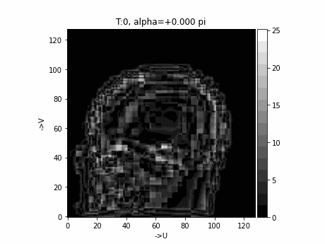
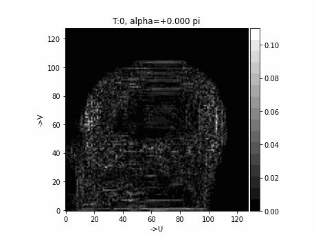
# Observe the colorbars. Note that the maximum value of the projection is
# around 60~, meaning a value of error of 14, is very relevant, while a
# value of error of 0.1 is less.

# geo.accuracy=3
tigre.plotproj(np.abs(projInterp3 - projInterp3001), angles)
# geo.accuracy=1
tigre.plotproj(np.abs(projInterp1 - projInterp3001), angles)
# geo.accuracy=0.5
tigre.plotproj(np.abs(projInterp05 - projInterp3001), angles)
# geo.accuracy=0.2
tigre.plotproj(np.abs(projInterp02 - projInterp3001), angles)
# geo.accuracy=0.05
tigre.plotproj(np.abs(projInterp3005 - projInterp3001), angles)

# From these plots we can conclude that  a value of 1 or less of
# geo.accuracy i srasonable. The smaller the better, but eventually the
# error will be so small that the imporvement is unperceptible. we
# recommend something in the range [0.1-0.5]
Total running time of the script: (0 minutes 1.482 seconds)