

Note
Go to the end to download the full example code.
Digital breast tomosynthesis#
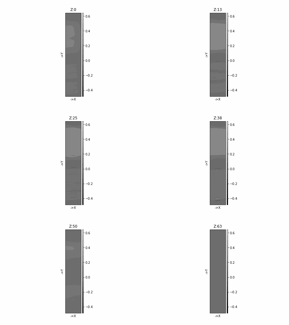
A limited-angle cone-beam scan, reconstructed with FDK and OS-SART.
Source: Python/demos/d19_DBTexample.py · MATLAB/Demos/d19_DBTexample.m
MATLAB version of this demo
clc;clear;close all
%%
%
% Code by Rodrigo Vimiero.
% https://github.com/rodrigovimieiro
%% Digital brest Thomosynthesis demo
%
% Few tricks to the geometry are needed to fix the detector in place.
% OTherwise its basic tomgoraphy.
%


%% Example
%
%
%
% VARIABLE                                   DESCRIPTION                    UNITS
%-------------------------------------------------------------------------------------
% Distances
geo.DSD = 660;                              % Distance Source Detector      (mm)
geo.DSO = 620;                              % Distance Source Origin        (mm)
% Detector parameters
geo.nDetector=[3064;2396]/2;					% number of pixels              (px)
geo.dDetector=[0.1; 0.1]; 					% size of each pixel            (mm)
geo.sDetector=geo.nDetector.*geo.dDetector; % total size of the detector    (mm)
% Image parameters
geo.nVoxel=[128;2054;784]/2;                  % number of voxels              (vx)
geo.sVoxel=[63.3;205.3;78.4]/2;               % total size of the image       (mm)
geo.dVoxel=geo.sVoxel./geo.nVoxel;          % size of each voxel            (mm)
% Offsets
Airgap = 22;                                % DBT airgap (mm)
geo.offOrigin =[((geo.sVoxel(1)/2)-...
    (geo.DSD-geo.DSO)+Airgap);0;geo.sVoxel(3)/2]; % Offset of image from origin (mm)
geo.offDetector=[0; geo.sDetector(2)/2];    % Offset of Detector            (mm)
% These two can be also defined
% per angle
% Auxiliary
geo.accuracy=0.5;                           % Variable to define accuracy of
% 'interpolated' projection
% It defines the amount of
% samples per voxel.
% Recommended <=0.5             (vx/sample)
% Optional Parameters
% There is no need to define these unless you actually need them in your
% reconstruction


geo.COR=0;                                  % y direction displacement for
% centre of rotation
% correction                   (mm)
% This can also be defined per
% angle
nprojs = 9;                                 % Number of projections
tubeangle = 25;                             % Angle range
angles=deg2rad(linspace(-tubeangle/2,tubeangle/2,nprojs)); % Angles in rad
geo.rotDetector=[0;0;0];                    % Rotation of the detector, by
% X,Y and Z axis respectively. (rad)
% This can also be defined per
% angle

geo.mode='cone';                            % Or 'parallel'. Geometry type.

%% Adapt CT geo to DBT
geo=staticDetectorGeo(geo,angles);
%% Adapt DBT projections to TIGRE CT projections

% Example of data (CT Head). This is not a true DBT, but it works as a
% example in TIGRE. Make sure to use a true tomosynthesis data.
head=headPhantom(geo.nVoxel);
projections=Ax(head,geo,angles,'interpolated');
% If you use a true DBT projection, use the following lines to adapt you
% data to TIGRE CT.Remember to use -log in your data.
% projections = -log(projections./single(2^14-1)); %your maximum white
% level.
%% Simple BP
recFDK = FDK( projections,geo,angles);

%% SART
recSART = SART(projections,geo,angles,2,'OrderStrategy','ordered');

%% plot
plotImg([recFDK recSART],'dim','x','clims',[0 1])
Initialize#
import tigre
import tigre.algorithms as algs
from tigre.utilities import sample_loader
from tigre.utilities.common_geometry import staticDetectorGeo
from tigre.utilities.geometry import Geometry
from tigre.utilities.geometry_default import ConeGeometryDefault

import numpy as np
from numpy import ndarray

def get_angles(tube_angle: int = 25, num_projections: int = 9) -> ndarray:
    angles = np.linspace(-tube_angle / 2, tube_angle / 2, num_projections)
    return np.radians(angles)

def get_geometry() -> ConeGeometryDefault:
    geo = tigre.geometry_default(high_resolution=False)
    pixel_mm, slice_mm = 0.1, 0.5
    row_pixels, col_pixels = 3064, 2396
    source_to_detector_mm = 660
    source_to_origin_mm = 620

    geo.DSD = source_to_detector_mm
    geo.DSO = source_to_origin_mm

    geo.nDetector = np.array(([row_pixels, col_pixels])) // 2
    geo.dDetector = np.array([pixel_mm, pixel_mm])
    geo.sDetector = geo.nDetector * geo.dDetector

    num_voxels_z, num_voxels_y, num_voxels_x = 128, 2054, 784
    geo.nVoxel = np.array([num_voxels_z, num_voxels_y, num_voxels_x]) // 2
    geo.sVoxel = np.array([num_voxels_z * slice_mm, num_voxels_y * pixel_mm, num_voxels_x * pixel_mm]) // 2
    geo.dVoxel = geo.sVoxel / geo.nVoxel

    airgap_mm = 22
    # These two can be also defined per angle auxiliary
    geo.offOrigin = np.array([geo.sVoxel[0] / 2 - (geo.DSD - geo.DSO) + airgap_mm, 0, geo.sVoxel[2]/2])
    geo.offDetector = np.array([0, geo.sDetector[1] / 2])

    # Variable to define accuracy of 'interpolated' projection.
    # It defines the amount of samples per voxel.
    # Recommended <=0.5 (vx/sample)
    geo.accuracy=0.5

    # Can also be defined per angle
    center_of_rotation_y_displacement_mm = 0.
    geo.COR = center_of_rotation_y_displacement_mm  # type: ignore

    # Rotation of the detector, by X,Y and Z axis respectively.
    # This can also be defined per angle.
    geo.rotDetector = np.array([0, 0, 0])
    geo.mode= "cone"  # Can be "parallel" as well
    return geo

def get_projections(geo: Geometry, angles: ndarray) -> ndarray:
    # Example data (CT Head). This is not a true DBT, but it works as an example.
    head = sample_loader.load_head_phantom(geo.nVoxel)
    projections = tigre.Ax(head, geo, angles, 'interpolated')
    # NOTE:
    # If you use a true DBT projection, use the following lines to adapt your data to TIGRE CT:
    # max_pixel_val = 2**14 - 1
    # projections = -np.log(projections / max_pixel_val)
    return projections

def compare_reconstruction_methods(projections: ndarray, geo: Geometry, angles: ndarray) -> None:
    imgFDK = algs.fdk(projections, geo, angles)

    num_iterations = 2
    imgOSSART = algs.ossart(projections, geo, angles, num_iterations)

    tigre.plotimg(np.concatenate([imgFDK, imgOSSART], axis=1), dim="z")

angles = get_angles()
geo = get_geometry()
geo = staticDetectorGeo(geo, angles)  # Adapt CT geo to DBT
projections = get_projections(geo, angles)
compare_reconstruction_methods(projections, geo, angles)
C:\Users\ander\anaconda3\envs\tigre\Lib\site-packages\tigre\utilities\parkerweight.py:34: UserWarning: Parker weights not supported for varying geo.DSD, mean(geo.DSD) is used.
  warnings.warn("Parker weights not supported for varying geo.DSD, mean(geo.DSD) is used.")
C:\Users\ander\anaconda3\envs\tigre\Lib\site-packages\tigre\utilities\parkerweight.py:51: UserWarning: Scanning angles smaller than pi+cone_angle. This is limited angle tomography,
there is no sufficient data, thus weighting for data redundancy is not required.
  warnings.warn(
OSSART algorithm in progress.
Estimated time until completion : 00:00:00
Algorithm will finish at        : 16:56:14
Total running time of the script: (0 minutes 12.572 seconds)