

Note
Go to the end to download the full example code.
Krylov subspace methods#
CGLS, LSQR, LSMR, hybrid LSQR and the GMRES variants.
Source: Python/demos/d08_Algorithms03.py · MATLAB/Demos/d08_Algorithms03.m
MATLAB version of this demo
%% DEMO 8:  Algorithms 03. Krylov subspace
%
%
% In this demo the usage of the the Krylov subspace family is explained.
% This family of algorithms iterates through the eigenvectors of the
% residual (Ax-b) of the problem in descending order, achieving increased
% convergence rates comparing to SART family.
%
% In cases where the data is good quality, SART type families tend to reach
% to a better image, but when the data gets very big, or has bad quality,
% CGLS is a good and fast algorithm
%--------------------------------------------------------------------------
%--------------------------------------------------------------------------
% This file is part of the TIGRE Toolbox
%
% Copyright (c) 2015, University of Bath and
%                     CERN-European Organization for Nuclear Research
%                     All rights reserved.
%
% License:            Open Source under BSD.
%                     See the full license at
%                     https://github.com/CERN/TIGRE/blob/master/LICENSE
%
% Contact:            tigre.toolbox@gmail.com
% Codes:              https://github.com/CERN/TIGRE/
% Coded by:           Ander Biguri
%--------------------------------------------------------------------------
%% Initialize
clear;
close all;

%% Define Geometry
geo=defaultGeometry('nVoxel',[128,128,128]','nDetector',[128,128]);

%% Load data and generate projections
% see previous demo for explanation
angles=linspace(0,2*pi,100);
head=headPhantom(geo.nVoxel);
projections=Ax(head,geo,angles,'interpolated');
projections=addCTnoise(projections);

%% Algorithhms
% these algorithms are showcased and referenced in the paper:
% "On Krylov Methods for Large Scale CBCT Reconstruction", M Sabate Landman
% et al. To be published.

niter=30;

% We also introduce a new feature in this demo too: the posibility to add the
% ground Truth image for error norms, if you have it. This is only for
% algorithm study, as in real situations you don't have this (otherwise no
% need for recon, right?) but its good to show performance and
% semiconvergence.

% SIRT, for comparison
[imgsirt,ressirt,errorsirt]=SIRT(projections,geo,angles,niter,'groundTruth',head);
% CGLS, traditional and mostly used Krylov algorithm
[imgcgls,rescgls,errcgls]=CGLS(projections,geo,angles,niter,'groundTruth',head);
% LSQR, stable version of CGLS
[imglsqr,reslsqr,errlsqr]=LSQR(projections,geo,angles,niter,'groundTruth',head);
% LSMR, a different krylov algorithm. It has Tikhonov regularization for
% stability, controled with the parameter 'lambda'
[imglsmr,reslsmr,errlsmr]=LSMR(projections,geo,angles,niter,'groundTruth',head,'lambda',0);
[imglsmr2,reslsmr2,errlsmr2]=LSMR(projections,geo,angles,niter,'groundTruth',head,'lambda',30);
% hybrid LSQR, a reorthogonalizing version of LSQR that can lead to better
% stability.
[imghlsqr,reshlsqr,errhlsqr]=hybrid_LSQR(projections,geo,angles,niter,'groundTruth',head);
% ABBA-GMRES are a set of algorithms that accept unmatched backprojectors,
% which TIGRE (and most CT libraries) have.
% read more at: "GMRES methods for tomographic reconstruction with an unmatched back projector",
% Per Christian Hansen, Ken Hayami, Keiichi Morikuni
[imgabgmres,resabgmres,errabgmres]=AB_GMRES(projections,geo,angles,niter,'groundTruth',head);
[imgbagmres,resbagmres,errbagmres]=BA_GMRES(projections,geo,angles,niter,'groundTruth',head);
% these can have other backprojectors, not just the standard ones. You can
% backproject with FDK for ultra-fast convergence, for example.
[imgabgmresfdk,resabgmresfdk,errabgmresfdk]=AB_GMRES(projections,geo,angles,niter,'groundTruth',head,'backprojector','FDK');
[imgbagmresfdk,resbagmresfdk,errbagmresfdk]=BA_GMRES(projections,geo,angles,niter,'groundTruth',head,'backprojector','FDK');

%% plot results
%
% Notice semiconvergence (this also happens with the other algorithms in
% other demos). i.e. residual goes down, but error goes up.
% Notice how LSMR with regularization doesn't suffer from this.
% Notice fast covnergence of ABBA with FDK backprojector, but not as good
% as the other algorithms after long iterations
% Notice that they are sometimes stopped early, due to divergence
% (unmatched backprojector+numerical issues)

% clean up data:
errorsirt(errorsirt==0)=nan;
errcgls(errcgls==0)=nan;
errlsqr(errlsqr==0)=nan;
errlsmr(errlsmr==0)=nan;
errlsmr2(errlsmr2==0)=nan;
errhlsqr(errhlsqr==0)=nan;
errabgmres(errabgmres==0)=nan;
errbagmres(errbagmres==0)=nan;
errabgmresfdk(errabgmresfdk==0)=nan;
errbagmresfdk(errbagmresfdk==0)=nan;
%% plots N1:
set(0,'defaultTextInterpreter','latex');
set(0,'DefaultTextFontName','Helvetica')
figure(1)
subplot(121)
semilogy(errorsirt/norm(head(:)),'linewidth',2);
hold on;
semilogy(errcgls/norm(head(:)),'linewidth',2);
semilogy(errlsqr/norm(head(:)),'linewidth',2);
semilogy(errlsmr/norm(head(:)),'linewidth',2);
semilogy(errlsmr2/norm(head(:)),'linewidth',2);
semilogy(errhlsqr/norm(head(:)),'linewidth',2);
semilogy(errabgmres/norm(head(:)),'linewidth',2);
semilogy(errbagmres/norm(head(:)),'linewidth',2);
semilogy(errabgmresfdk/norm(head(:)),'linewidth',2);
semilogy(errbagmresfdk/norm(head(:)),'linewidth',2);
xlim([1,niter]);
ylim([7*10^-2,10^0])
xlabel("Iteration number")
ylabel("$\|x-x_{gt}\|/\|x_{gt}\|$",'interpreter','latex')
title("Error norm")
legend(["SIRT","CGLS","LSQR","LSMR $\lambda=0$","LSMR $\lambda=30$","hybrid LSQR","AB-GMRES","BA-GMRES","AB-GRMES ($B_{FDK}$)","BA-GRMES ($B_{FDK}$)"],'NumColumns',2,'interpreter','latex')

% set(gca,'fontsize',16)
set(gcf, 'Color', 'w');
grid on

subplot(122)

semilogy(ressirt/norm(projections(:)),'linewidth',2);
hold on;
semilogy(rescgls/norm(projections(:)),'linewidth',2);
semilogy(reslsqr/norm(projections(:)),'linewidth',2);
semilogy(reslsmr/norm(projections(:)),'linewidth',2);
semilogy(reslsmr2/norm(projections(:)),'linewidth',2);
semilogy(reshlsqr/norm(projections(:)),'linewidth',2);

semilogy(resabgmres/norm(projections(:)),'linewidth',2);
semilogy(resbagmres/norm(projections(:)),'linewidth',2);
semilogy(resabgmresfdk/norm(projections(:)),'linewidth',2);
semilogy(resbagmresfdk/norm(projections(:)),'linewidth',2);
xlim([1,niter]);
ylim([9*10^-3,10^0])
xlabel("Iteration number")
ylabel("$\|Ax-b\|/\|b\|$",'interpreter','latex')
title("Residual norm")
legend(["SIRT","CGLS","LSQR","LSMR $\lambda=0$","LSMR $\lambda=30$","hybrid LSQR","AB-GMRES","BA-GMRES","AB-GRMES ($B_{FDK}$)","BA-GRMES ($B_{FDK}$)"],'NumColumns',2,'interpreter','latex')
grid on
set(gcf, 'Color', 'w');
set(gcf, 'Units', 'Inches', 'Position', [1, 1, 15/1.2, 7/1.2], 'PaperUnits', 'Inches', 'PaperSize', [9/1.2 7/1.2])
% set(gca,'fontsize',16)
set(0,'defaultTextInterpreter','tex');

%% Hybrid methods with different regularization parameter choices

% you can explicitly defined the parameter in the mathematical terms
[imghLSQR_l10, residual_hLSQR_l10]=hybrid_LSQR(projections,geo,angles,30, 'lambda', 10);
% You can give it a "noise level" (in %) instead, and it will chose the lamba inside
[imghLSQR_nl002, residual_hLSQR_nl002,~, lambda_vec_nl002]=hybrid_LSQR(projections,geo,angles,30, 'NoiseLevel', 0.02);
% if you don't give it any, it will use Generalized Cross Validation to approximate a good lambda
[imghLSQR_gcv, residual_hLSQR_gcv,~, lambda_vec_gcv]=hybrid_LSQR(projections,geo,angles,30);

%% plot images
plotImg([imgcgls imghLSQR_l10 imghLSQR_nl002 imghLSQR_gcv],'Dim','Z','Step',2)

% Look at the parameters
figure
plot(lambda_vec_nl002)
hold on
plot(lambda_vec_gcv)
title("lambda vs iteratios")
legend(["Noise Level", "Generalized Cross Validation"])

%%
Initialize#
import tigre
import numpy as np
from tigre.utilities import sample_loader
from tigre.utilities import CTnoise
import tigre.algorithms as algs
from matplotlib import pyplot as plt
Geometry#
geo = tigre.geometry_default(high_resolution=False)
Load data and generate projections#
# define angles
angles = np.linspace(0, 2 * np.pi, 100, endpoint=False)
# Load thorax phantom data
head = sample_loader.load_head_phantom(geo.nVoxel)
# generate projections
projections = tigre.Ax(head, geo, angles)
# add noise
noise_projections = CTnoise.add(projections, Poisson=1e5, Gaussian=np.array([0, 10]))
Usage CGLS#
#
#
#  CGLS has the common 4 inputs for iterative algorithms in TIGRE:
#
#  Projections, geometry, angles, and number of iterations
#
# Additionally it contains optional initialization techniques, but we
# recommend not using them. CGLS is already quite fast and using them may
# lead to divergence.
# The options are:
#  'init'    Describes different initialization techniques.
#             -  'none'     : Initializes the image to zeros (default)
#             -  'FDK'      : initializes image to FDK reconstruction
#             -  'multigrid': Initializes image by solving the problem in
#                            small scale and increasing it when relative
#                            convergence is reached.
#             -  'image'    : Initialization using a user specified
#                            image. Not recommended unless you really
#                            know what you are doing.
#  'initimg'    an image for the 'image' initialization. Avoid.

# # use CGLS
imgCGLS, normL2CGLS = algs.cgls(noise_projections, geo, angles, 30, computel2=True)
# use LSQR
imgLSQR, normL2LSQR = algs.lsqr(noise_projections, geo, angles, 30, computel2=True)
# use LSMR
imgLSMR, normL2LSMR = algs.lsmr(noise_projections, geo, angles, 30, computel2=True,lmbda=0)
imgLSMR2, normL2LSMR2 = algs.lsmr(noise_projections, geo, angles, 30, computel2=True,lmbda=30)
# use hybrid LSQR
imghLSQR, normhL2LSQR = algs.hybrid_lsqr(noise_projections, geo, angles, 30, computel2=True)

# AB/BA-GMRES
imgabgmres, normhabgmres = algs.ab_gmres(noise_projections, geo, angles, 30, computel2=True)
imgbagmres, normhbagmres = algs.ba_gmres(noise_projections, geo, angles, 30, computel2=True)
# # AB/BA-GMRES with FDK backprojector
imgabgmresfdk, normhabgmresfdk = algs.ab_gmres(noise_projections, geo, angles, 30, computel2=True,backprojector="FDK")
imgbagmresfdk, normhbagmresfdk = algs.ba_gmres(noise_projections, geo, angles, 30, computel2=True,backprojector="FDK")

# SIRT for comparison.
imgSIRT, normL2SIRT = algs.sirt(noise_projections, geo, angles, 60, computel2=True)
CGLS algorithm in progress.
Estimated time until completion : 00:00:00
Algorithm will finish at        : 16:49:53
re-initilization of CGLS called at iteration:21
Average time taken for each iteration for CGLS:0.008052303224817038(s)
LSQR algorithm in progress.
Estimated time until completion : 00:00:00
Algorithm will finish at        : 16:49:54
LSMR algorithm in progress.
Estimated time until completion : 00:00:00
Algorithm will finish at        : 16:49:55
LSMR algorithm in progress.
Estimated time until completion : 00:00:00
Algorithm will finish at        : 16:49:56
HYBRID_LSQR algorithm in progress.
Estimated time until completion : 00:00:01
Algorithm will finish at        : 16:49:57
AB_GMRES algorithm in progress.
Estimated time until completion : 00:00:02
Algorithm will finish at        : 16:50:01
BA_GMRES algorithm in progress.
Estimated time until completion : 00:00:00
Algorithm will finish at        : 16:50:08
AB_GMRES algorithm in progress.
Estimated time until completion : 00:00:02
Algorithm will finish at        : 16:50:12
BA_GMRES algorithm in progress.
Estimated time until completion : 00:00:02
Algorithm will finish at        : 16:50:34
BA-GMRES exited due to divergence at iteration 13
SIRT algorithm in progress.
Estimated time until completion : 00:00:01
Algorithm will finish at        : 16:50:34
plot results#
#
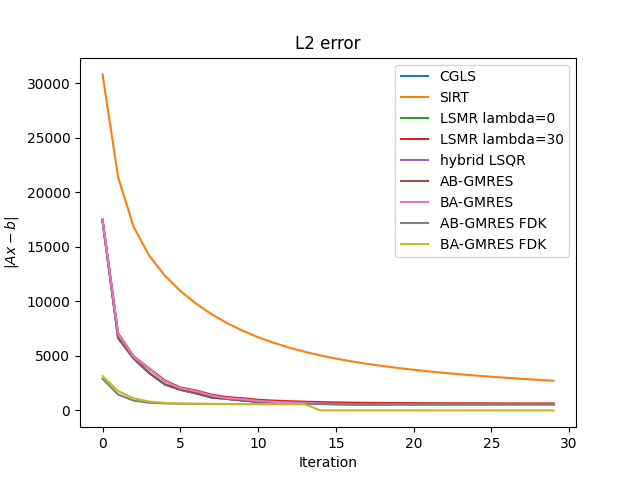
# We can see that CGLS gets to the same L2 error in less amount of
# iterations.

plt.plot(np.vstack((normL2CGLS[0, :], normL2SIRT[0, 0:30],normL2LSMR[0, :],normL2LSMR2[0, :],normhL2LSQR[0, :],normhabgmres[0,:],normhbagmres[0,:],normhabgmresfdk[0,:],normhbagmresfdk[0,:])).T)
plt.title("L2 error")
plt.xlabel("Iteration")
plt.ylabel("$ |Ax-b| $")
plt.gca().legend(("CGLS","SIRT","LSMR lambda=0","LSMR lambda=30","hybrid LSQR","AB-GMRES","BA-GMRES","AB-GMRES FDK","BA-GMRES FDK"))
plt.show()
# plot images
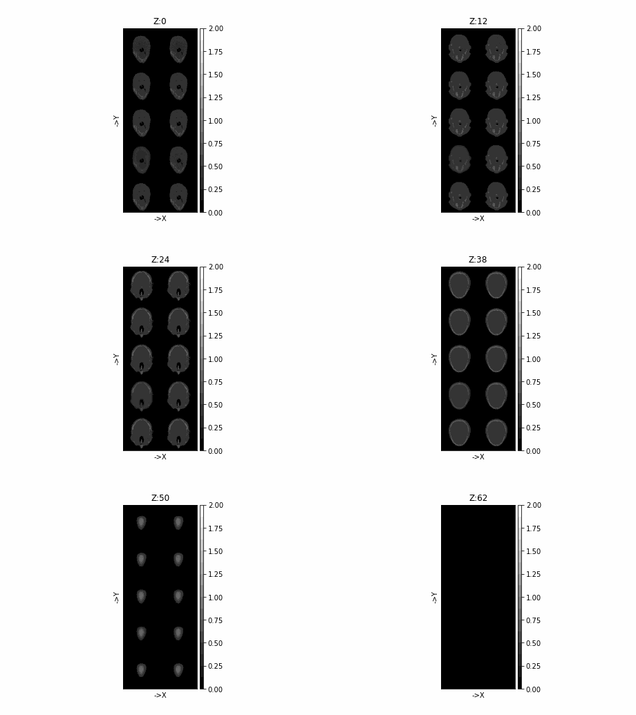
tigre.plotimg(np.concatenate([np.concatenate([imgCGLS, imgSIRT, imgLSQR,imgabgmres,imgabgmresfdk],axis=1),np.concatenate([imgLSMR, imgLSMR2, imghLSQR, imgbagmres, imgbagmresfdk], axis=1)], axis=2), dim="z", step=2, clims=[0, 2])
# plot errors
tigre.plotimg(np.concatenate([np.concatenate([head-imgCGLS, head-imgSIRT, head-imgLSQR, head-imgabgmres, head-imgabgmresfdk],axis=1),np.concatenate([head-imgLSMR, head-imgLSMR2, head-imghLSQR, head-imgbagmres, head-imgbagmresfdk], axis=1)], axis=2), dim="z", slice=32)
Total running time of the script: (0 minutes 44.372 seconds)