

Note
Go to the end to download the full example code.
SART, OS-SART and SIRT#
The SART family, the options they share, and how they compare.
Source: Python/demos/d07_Algorithms02.py · MATLAB/Demos/d07_Algorithms02.m
MATLAB version of this demo
%% DEMO 7:  Algorithms 02. SART
%
%
% In this demo the usage of the algorithms on the SART family among with
% their options are presented.
%
%
%--------------------------------------------------------------------------
%--------------------------------------------------------------------------
% This file is part of the TIGRE Toolbox
%
% Copyright (c) 2015, University of Bath and
%                     CERN-European Organization for Nuclear Research
%                     All rights reserved.
%
% License:            Open Source under BSD.
%                     See the full license at
%                     https://github.com/CERN/TIGRE/blob/master/LICENSE
%
% Contact:            tigre.toolbox@gmail.com
% Codes:              https://github.com/CERN/TIGRE/
% Coded by:           Ander Biguri
%--------------------------------------------------------------------------
%% Initialize
clear;
close all;

%% Define Geometry
geo=defaultGeometry('nVoxel',[128;128;128]);

%% Load data and generate projections
% see previous demo for explanation
angles=linspace(0,2*pi,100);
head=headPhantom(geo.nVoxel);
projections=Ax(head,geo,angles,'interpolated');
noise_projections=addCTnoise(projections);
%% SART family of algorithms
%
% There are 3 algorithms in this damily included in TIGRE: SART,SIRT and
% OS-SART.
%
% The main difference between them is the update process.
%   SART: Updates the image projection by projection
%   SIRT: Updates the image using the whole set of projections at once
%   OS-SART: middle ground. Updates the image using a subset of the
%            projections
%
%  Of these algorithms, SART is generally the one reaching a better image
%  (less L2 error) for the same amount of iterations, and SIRT is the
%  worst (still relatively similar). However, SART needs increased
%  computational time per iteration, as it needs to update the image very often,
%  while SIRT only updates the image once for the whole set of projections.
%  OS-SART lies in the middle, reaching similar convergence (L2 error per
%  iteration) than SART but with less computational time than SART.
%
%% Usage, with optional parameters.
% In the three algorithms, there are 4 mandatory input arguments:
% Projections, geometry, angles and number of iterations.
%
%
% Optional arguments for all of them
%==========================================================================
% 'lambda': hyperparameter. The update will be multiplied by this number
% every iteration, to make the steps bigger or smaller. Default: 1
%
lambda=1;


% 'lambdared': reduction multiplier for the hyperparameter.
% lambda=lambda*lambdared every iteration, so the steps can be smaller
% the further the update. Default=0.99
lambdared=0.999;

% 'Init' : Initialization method. Possible options are
%          'none' (default). There will be no initialization method, just
%                 the algorithm
%
%          'FDK'  Initialize the image with the result of FDK algorithm
%
%          'multigrid' Initialize using the multigrid method. The image
%                      will be solved in a small scale, and the size of it
%                      will increase until the desired size is reached.
%
%          'image'     Initializes with a user given image. Not recommended
%                      unless you really know what you are doing.

initmode='none';

% 'InitImg' : related to init. The image to use for initializing the
% algorithm.

% 'verbose': boolean to make the algorithm display (or not) running state.
%            default true.

verbose=true;
% 'QualMeas'     Asks the algorithm for a set of quality measurement
%                parameters. Input should contain a cell array of desired
%                quality measurement names. Example: {'CC','RMSE','MSSIM'}
%                These will be computed in each iteration.
qualmeas={'RMSE'};

% SIRT and SART both have no extra input parameters.
% =========================================================================
[imgSIRT,errL2SIRT,qualitySIRT]=SIRT(projections,geo,angles,20,...
                            'lambda',lambda,'lambda_red',lambdared,'verbose',verbose,'QualMeas',qualmeas);
[imgSART,errL2SART,qualitySART]=SART(projections,geo,angles,20,...
                            'lambda',lambda,'lambda_red',lambdared,'verbose',verbose,'QualMeas',qualmeas);
% OS-SART
% ========================================================================
% Additionally OS-SART includes a couple of other parameters, related to
% the subsets.
%
%   'BlockSize':   Sets the projection block size used simultaneously. If
%                  BlockSize = 1 OS-SART becomes SART and if  BlockSize = size(angles,2)
%                  then OS-SART becomes SIRT. Default is 20.
blcks=8;
% 'OrderStrategy':  Chooses the subset ordering strategy. Options are
%                  'ordered' :uses them in the input order, but divided
%                  'random'  : orders them randomly
%                  'angularDistance': chooses the next subset with the
%                                     biggest angular distance with the
%                                     ones used.  (default)
order='angularDistance';
[imgOSSART,errL2OSSART,qualityOSSART]=OS_SART(projections,geo,angles,20,...
                            'lambda',lambda,'lambda_red',lambdared,'verbose',verbose,'QualMeas',qualmeas,...
                             'BlockSize',blcks,'OrderStrategy',order);
%% Lets have a brief show of the results
% set(0,'DefaultTextInterpreter', 'latex')

subplot(211)
plot(log10([errL2SIRT;[errL2OSSART nan(1,length(errL2SIRT)-length(errL2OSSART))];[errL2SART nan(1,length(errL2SIRT)-length(errL2SART))]]'));
title('Convergence')
xlabel('Iteration')
ylabel('$ log_{10}(|Ax-b|) $','interpreter','latex')
legend('SIRT','OS-SART','SART')
subplot(212)
plot(log10([qualitySIRT;[qualityOSSART nan(1,length(qualitySIRT)-length(qualityOSSART))];[qualitySART nan(1,length(qualitySIRT)-length(qualitySART))]]'));
title('Evolution of RMSE')
legend('SIRT','OS-SART','SART')
xlabel('Iteration')
ylabel('$ log_{10}(RMSE) $','interpreter','latex')

%% plot the results

% It is clear that SART will get to better results for the same amount of
% iterations, however, it takes x7 more time to run.

% SART
% OS-SART
% SIRT

plotImg([imgSIRT;  imgOSSART; imgSART;],'Dim','Z','Savegif','sarts.gif');

% plot error
plotImg(abs([head-imgSIRT; head-imgOSSART; head-imgSART; ]),'Dim','Z');
Initialize#
import tigre
import numpy as np
from tigre.utilities import sample_loader
from tigre.utilities import CTnoise
import tigre.algorithms as algs
from matplotlib import pyplot as plt
Geometry#
geo = tigre.geometry_default(high_resolution=False)
Load data and generate projections#
# define angles
angles = np.linspace(0, 2 * np.pi, 100, endpoint=False)
# Load thorax phantom data
head = sample_loader.load_head_phantom(geo.nVoxel)
# generate projections
projections = tigre.Ax(head, geo, angles)
# add noise
noise_projections = CTnoise.add(projections, Poisson=1e5, Gaussian=np.array([0, 10]))
Algorithms#
#
# The main difference between them is the update process.
#   SART: Updates the image projection by projection
#   SIRT: Updates the image using the whole set of projections at once
#   OS-SART: middle ground. Updates the image using a subset of the
#            projections
#
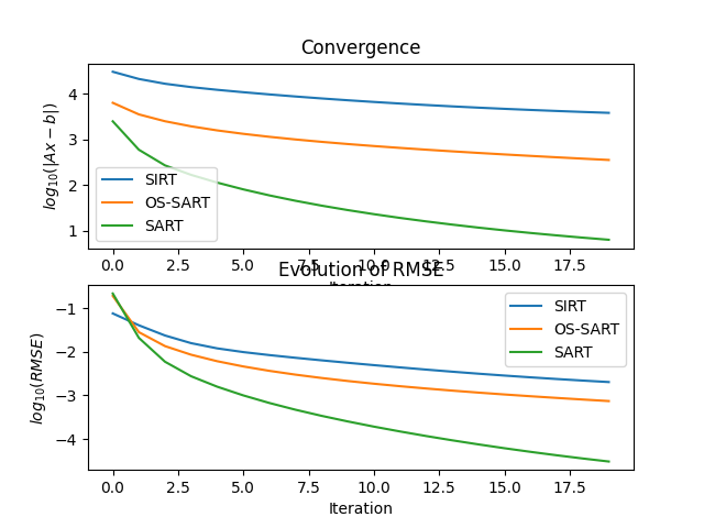
#  Of these algorithms, SART is generally the one reaching a better image
#  (less L2 error) for the same amount of iterations, and SIRT is the
#  worst (still relatively similar). However, SART needs increased
#  computational time per iteration, as it needs to update the image very often,
#  while SIRT only updates the image once for the whole set of projections.
#  OS-SART lies in the middle, reaching similar convergence (L2 error per
#  iteration) than SART but with less computational time than SART.
#
## Usage, with optional parameters.
# In the three algorithms, there are 4 mandatory input arguments:
# Projections, geometry, angles and number of iterations.
#
#
# Optional arguments for all of them
# ==========================================================================
# 'lmbda': hyperparameter (lambda). The update will be multiplied by this
# number every iteration, to make the steps bigger or smaller. Default: 1
#
lmbda = 1

# 'lmbda_red': reduction multiplier for the hyperparameter.
# lmbda=lmbda*lmbda_red every iteration, so the steps can be smaller
# the further the update. Default=0.99
lambdared = 0.999

# 'init' : Initialization method. Possible options are
#          None (default). There will be no initialization method, just
#                 the algorithm
#
#          'FDK'  Initialize the image with the result of FDK algorithm
#
#          'multigrid' Initialize using the multigrid method. The image
#                      will be solved in a small scale, and the size of it
#                      will increase until the desired size is reached.
#
#          'image'     Initializes with a user given image. Not recommended
#                      unless you really know what you are doing.

initmode = None

# 'initimg' : related to init. The image to use for initializing the
# algorithm.

# 'verbose': boolean to make the algorithm display (or not) running state.
#            default true.

verbose = True
# 'Quameasopts'  Asks the algorithm for a set of quality measurement
#                parameters. Input should contain a list of desired
#                quality measurement names. Example: ['CC','RMSE','MSSIM']
#                These will be computed in each iteration.
#                Note that this is the change in parameter value per iteration, not the quality of the result.
qualmeas = ["RMSE", "SSD"]

# SIRT and SART both have no extra input parameters.
# =========================================================================
imgSIRT, qualitySIRT = algs.sirt(
    projections,
    geo,
    angles,
    20,
    lmbda=lmbda,
    lmbda_red=lambdared,
    verbose=verbose,
    Quameasopts=qualmeas,
    computel2=True,
)
imgSART, qualitySART = algs.sart(
    projections,
    geo,
    angles,
    20,
    lmbda=lmbda,
    lmbda_red=lambdared,
    verbose=verbose,
    Quameasopts=qualmeas,
    computel2=True,
)

# OS-SART
# ========================================================================
# Additionally OS-SART includes a couple of other parameters, related to
# the subsets.
#
#   'blocksize':   Sets the projection block size used simultaneously. If
#                  BlockSize = 1 OS-SART becomes SART and if  BlockSize = size(angles,2)
#                  then OS-SART becomes SIRT. Default is 20.
blcks = 10
# 'OrderStrategy':  Chooses the subset ordering strategy. Options are
#                  'ordered' :uses them in the input order, but divided
#                  'random'  : orders them randomly
#                  'angularDistance': chooses the next subset with the
#                                     biggest angular distance with the
#                                     ones used.  (default)
order = "random"
imgOSSART, qualityOSSART = algs.ossart(
    projections,
    geo,
    angles,
    20,
    lmbda=lmbda,
    lmbda_red=lambdared,
    verbose=verbose,
    Quameasopts=qualmeas,
    blocksize=blcks,
    OrderStrategy=order,
    computel2=True,
)
SIRT algorithm in progress.
Estimated time until completion : 00:00:01
Algorithm will finish at        : 16:49:22
SART algorithm in progress.
Estimated time until completion : 00:00:11
Algorithm will finish at        : 16:49:34
OSSART algorithm in progress.
Estimated time until completion : 00:00:01
Algorithm will finish at        : 16:49:37
Lets have a brief show of the results#
plt.subplot(211)
plt.plot(np.log10(np.vstack((qualitySIRT[0, :], qualityOSSART[0, :], qualitySART[0, :]))).T)
plt.title("Convergence")
plt.xlabel("Iteration")
plt.ylabel("$ log_{10}(|Ax-b|) $")
plt.gca().legend(("SIRT", "OS-SART", "SART"))
plt.subplot(212)
plt.plot(np.log10(np.vstack((qualitySIRT[1, :], qualityOSSART[1, :], qualitySART[1, :]))).T)
plt.title("Evolution of RMSE")
plt.gca().legend(("SIRT", "OS-SART", "SART"))
plt.xlabel("Iteration")
plt.ylabel("$ log_{10}(RMSE) $")
plt.show()
plot the results#
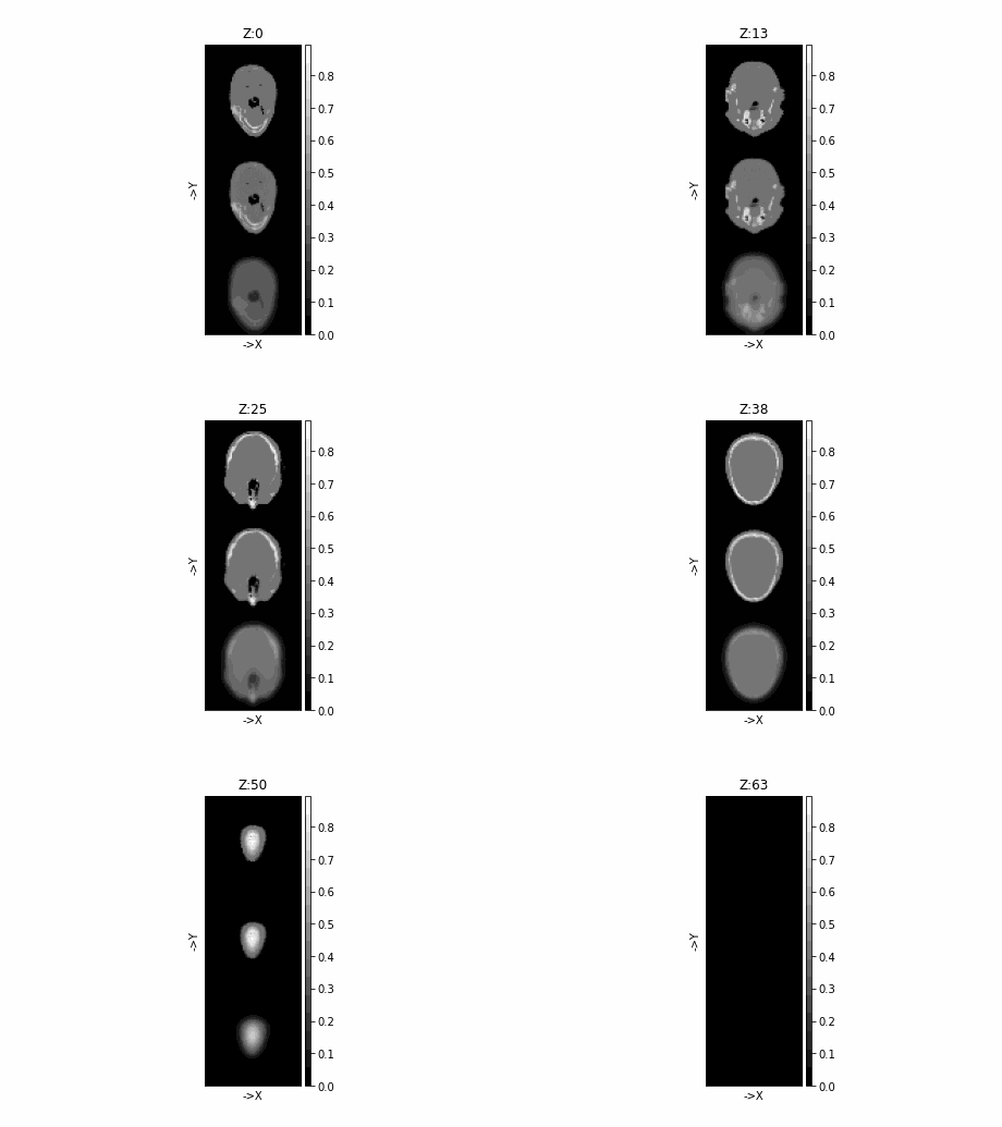
# It is clear that SART will get to better results for the same amount of
# iterations, however, it takes x7 more time to run.

# SART
# OS-SART
# SIRT

tigre.plotimg(np.concatenate([imgSIRT, imgOSSART, imgSART], axis=1), dim="Z", savegif="sarts.gif")

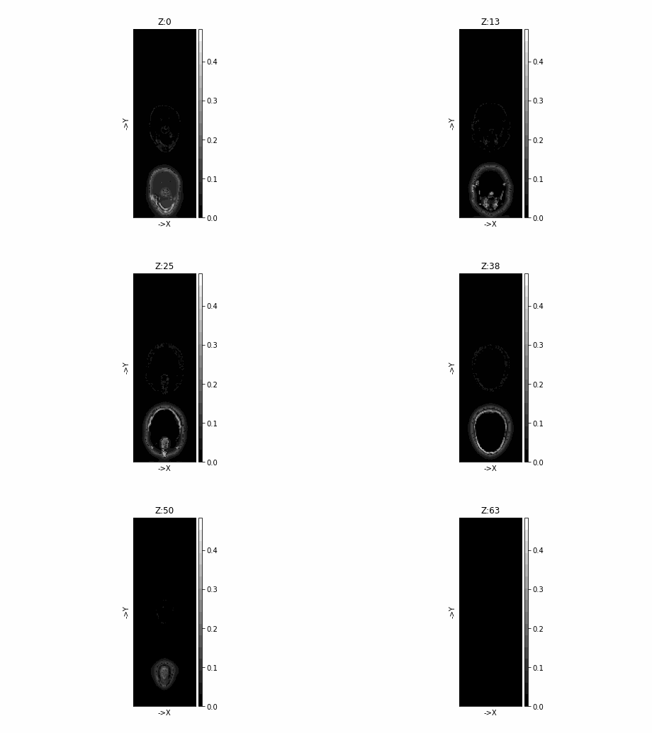
# plot error
tigre.plotimg(
    np.abs(np.concatenate([head - imgSIRT, head - imgOSSART, head - imgSART], axis=1)), dim="Z"
)
Total running time of the script: (0 minutes 31.902 seconds)