

Note
Go to the end to download the full example code.
FDK and its filters#
Filtered backprojection for cone beam, with the available filters.
Source: Python/demos/d06_Algorithms01.py · MATLAB/Demos/d06_Algorithms01.m
MATLAB version of this demo
%% DEMO 6:  Algorithms 01.
%
%
% In this demo the usage of the FDK is explained
%
%
%--------------------------------------------------------------------------
%--------------------------------------------------------------------------
% This file is part of the TIGRE Toolbox
%
% Copyright (c) 2015, University of Bath and
%                     CERN-European Organization for Nuclear Research
%                     All rights reserved.
%
% License:            Open Source under BSD.
%                     See the full license at
%                     https://github.com/CERN/TIGRE/blob/master/LICENSE
%
% Contact:            tigre.toolbox@gmail.com
% Codes:              https://github.com/CERN/TIGRE/
% Coded by:           Ander Biguri
%--------------------------------------------------------------------------
%% Initialize
clear;
close all;

%% Define Geometry
geo=defaultGeometry('nVoxel',[128;128;128]);

%% Load data and generate projections
% see previous demo for explanation
angles=linspace(0,2*pi,200);
head=headPhantom(geo.nVoxel);
projections=Ax(head,geo,angles,'interpolated');
noise_projections=addCTnoise(projections);

%% Usage of FDK

% the FDK algorithm has been taken and modified from
% 3D Cone beam CT (CBCT) projection backprojection FDK, iterative reconstruction Matlab examples
% https://www.mathworks.com/matlabcentral/fileexchange/35548-3d-cone-beam-ct--cbct--projection-backprojection-fdk--iterative-reconstruction-matlab-examples

% The algorithm takes, as any of them, 3 mandatory inputs:
% PROJECTIONS: Projection data
% GEOMETRY   : Geometry describing the system
% ANGLES     : Projection angles
% And has a single optional argument:
% FILTER: filter type applied to the projections. Possible options are
%        'ram-lak' (default)
%        'shepp-logan'
%        'cosine'
%        'hamming'
%        'hann'
% The choice of filter will modify the noise and some discretization
% errors, depending on which is chosen.
%
imgFDK1=FDK(noise_projections,geo,angles,'filter','hann');
imgFDK2=FDK(noise_projections,geo,angles,'filter','ram-lak');


% They look quite the same
plotImg([imgFDK1 imgFDK2],'Dim','Z');

% but it can be seen that one has bigger errors in the whole image, while
% the other just in the boundaries
plotImg([abs(head-imgFDK1) abs(head-imgFDK2)],'Dim','Z');
Initialize#
import tigre
import numpy as np
from tigre.utilities import sample_loader
from tigre.utilities import CTnoise
import tigre.algorithms as algs
Geometry#
geo = tigre.geometry_default(high_resolution=False)
Load data and generate projections#
# define angles
angles = np.linspace(0, 2 * np.pi, 100, endpoint=False)
# Load thorax phantom data
head = sample_loader.load_head_phantom(geo.nVoxel)
# generate projections
projections = tigre.Ax(head, geo, angles)
# add noise
noise_projections = CTnoise.add(projections, Poisson=1e5, Gaussian=np.array([0, 10]))
Usage of FDK#
# the FDK algorithm has been taken and modified from
# 3D Cone beam CT (CBCT) projection backprojection FDK, iterative reconstruction Matlab examples
# https://www.mathworks.com/matlabcentral/fileexchange/35548-3d-cone-beam-ct--cbct--projection-backprojection-fdk--iterative-reconstruction-matlab-examples

# The algorithm takes, as any of them, 3 mandatory inputs:
# PROJECTIONS: Projection data
# GEOMETRY   : Geometry describing the system
# ANGLES     : Projection angles
# And has a single optional argument:
# FILTER: filter type applied to the projections. Possible options are
#        'ram_lak' (default)
#        'shepp_logan'
#        'cosine'
#        'hamming'
#        'hann'
# The choice of filter will modify the noise and some discretization
# errors, depending on which is chosen.
#
imgFDK1 = algs.fdk(noise_projections, geo, angles, filter="hann")
imgFDK2 = algs.fdk(noise_projections, geo, angles, filter="ram_lak")

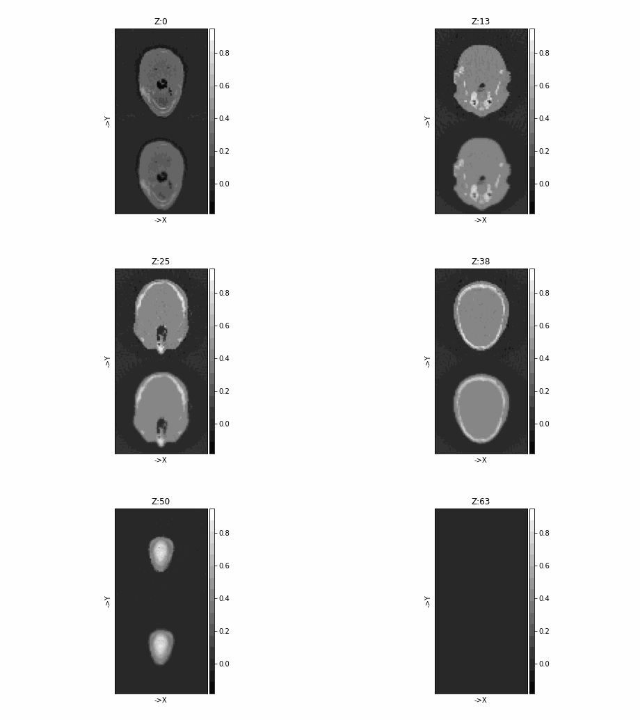
# They look quite the same
tigre.plotimg(np.concatenate([imgFDK1, imgFDK2], axis=1), dim="Z")

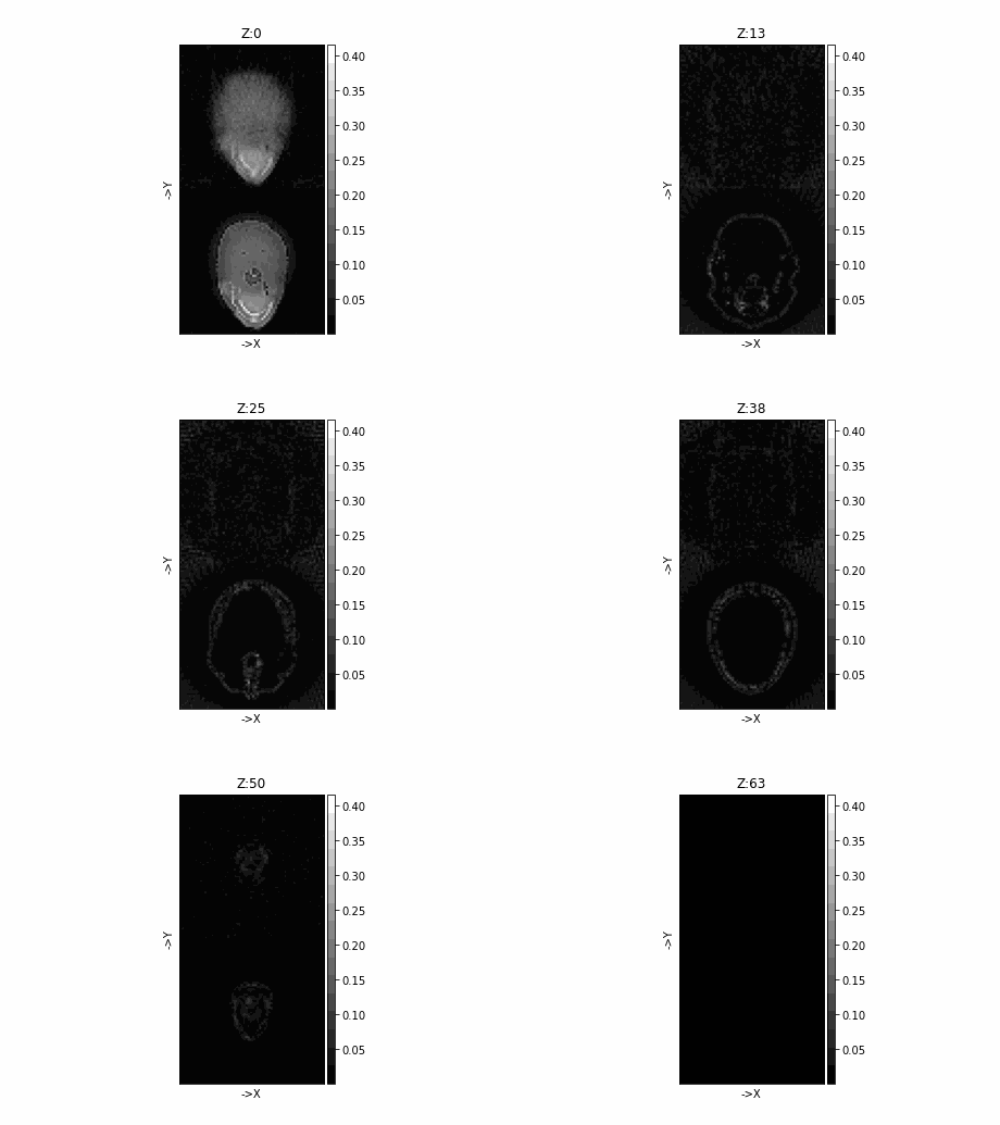
# but it can be seen that one has bigger errors in the whole image, while
# the other just in the boundaries
tigre.plotimg(np.concatenate([abs(head - imgFDK1), abs(head - imgFDK2)], axis=1), dim="Z")
Total running time of the script: (0 minutes 8.566 seconds)