

Note
Go to the end to download the full example code.
Helical scans#
Move the image along the rotation axis at each angle.
Source: Python/demos/d13_HelicalGeometry.py · MATLAB/Demos/d13_HelicalGeometry.m
MATLAB version of this demo
%% Demo 13: Helical Geometry tests
%
%
% This demo shows an example of TIGRE working on Helical scan geometries
%
%--------------------------------------------------------------------------
%--------------------------------------------------------------------------
% This file is part of the TIGRE Toolbox
%
% Copyright (c) 2015, University of Bath and
%                     CERN-European Organization for Nuclear Research
%                     All rights reserved.
%
% License:            Open Source under BSD.
%                     See the full license at
%                     https://github.com/CERN/TIGRE/blob/master/LICENSE
%
% Contact:            tigre.toolbox@gmail.com
% Codes:              https://github.com/CERN/TIGRE/
% Coded by:           Ander Biguri
%--------------------------------------------------------------------------
%%

clear;
clc;

geo.DSD = 1536;                             % Distance Source Detector      (mm)
geo.DSO = 1000;                             % Distance Source Origin        (mm)
% Detector parameters
geo.nDetector=[512; 512];					% number of pixels              (px)
geo.dDetector=[0.8; 0.8]; 					% size of each pixel            (mm)
geo.sDetector=geo.nDetector.*geo.dDetector; % total size of the detector    (mm)
% Image parameters
geo.nVoxel=[128;128;512];                   % number of voxels              (vx)
geo.sVoxel=[256;256;1024];                   % total size of the image       (mm)
geo.dVoxel=geo.sVoxel./geo.nVoxel;          % size of each voxel            (mm)
% Offsets
geo.offDetector=[0; 0];                     % Offset of Detector            (mm)
geo.COR=0;
geo.mode='cone';

% Auxiliary
geo.accuracy=0.5;


%% Create data+ angles
angles=linspace(0.0,2*pi,100);
angles=[angles angles angles]; % 3 rotations
% Load thorax phantom data
head=headPhantom(geo.nVoxel); % yes, not the best example data, but It will do.

% This makes it helical
geo.offOrigin(3,:)=linspace(-1024/2+128,1024/2-128,size(angles,2)).';  % about 256^3 images fit in the detector with this size.
geo.offOrigin(1,:)=0;
geo.offOrigin(2,:)=0;

% project data
data=Ax(head,geo,angles);

% Uncomment if you want to see the data
%plotProj(data,angles);
%% Reconstruct Helical

OSSARTimg=OS_SART(data,geo,angles,30);
% SARTimg=SART(data,geo,angles,30); % takes time
CGLSimg=CGLS(data,geo,angles,20); %% Plot results

% CGLS and SIRT
plotImg([head, OSSARTimg ,CGLSimg],'Dim',3,'Step',3);
Initialize#
import tigre
import numpy as np
from tigre.utilities import sample_loader
import tigre.algorithms as algs
import time
Geometry#
geo = tigre.geometry_default(high_resolution=False)

angles = np.linspace(0, 2 * np.pi, 100, endpoint=False)
angles = np.hstack([angles, angles, angles])  # loop 3 times

# Load thorax phantom data
head = sample_loader.load_head_phantom(geo.nVoxel)

# This makes it helical.
#
# NOTE the component ordering: the Python bindings map offOrigin as
# (z, y, x) - matching numpy's volume index order - so the axial (helix)
# motion goes in column 0. This differs from MATLAB, whose offOrigin is
# (x, y, z) and whose version of this demo therefore uses offOrigin(3,:).
# Porting by keeping the index silently translates the volume along the
# BEAM instead of along the rotation axis.
geo.offOrigin = np.zeros((angles.shape[0], 3))
geo.offOrigin[:, 0] = np.linspace(
    -1024 / 2 + 128, 1024 / 2 - 128, angles.shape[0]
)  # about 256^3 images fit int he detector with this size.

# project data
data = tigre.Ax(head, geo, angles)

# Uncomment if you want to see the data
# plotProj(data,angles);
## Reconstruct Helical

SIRTimg = algs.sirt(data, geo, angles, 30)
# SARTimg=SART(data,geo,angles,30); # takes time
CGLSimg = algs.cgls(data, geo, angles, 20)
## Plot results

# CGLS and SIRT
tigre.plotImg(np.concatenate([head, SIRTimg, CGLSimg], axis=1), dim="z", step=3, clims=[0, 1])
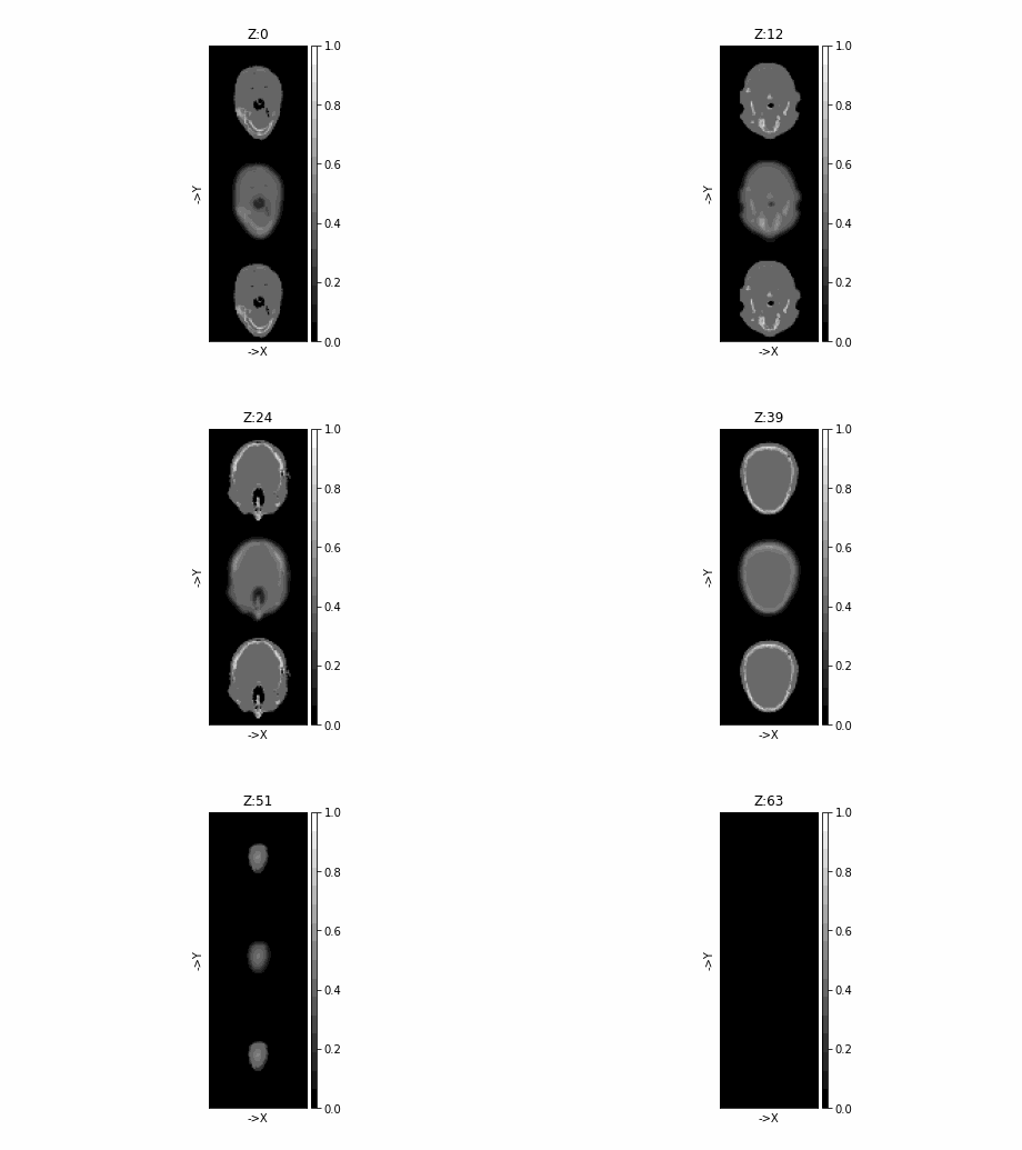
SIRT algorithm in progress.
Estimated time until completion : 00:00:03
Algorithm will finish at        : 16:51:21
CGLS algorithm in progress.
Estimated time until completion : 00:00:01
Algorithm will finish at        : 16:51:20
Average time taken for each iteration for CGLS:0.026790394998533883(s)
Total running time of the script: (0 minutes 5.054 seconds)