

Note
Go to the end to download the full example code.
Parallel-beam geometry#
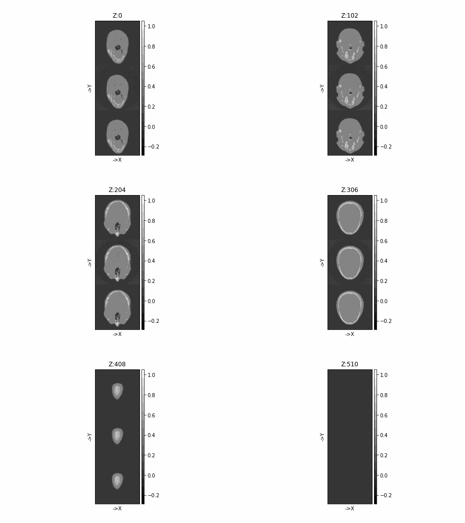
Reconstruct 3D parallel-beam data, as from a synchrotron.
Source: Python/demos/d15_3Dparallel.py · MATLAB/Demos/d15_3Dparallel.m
MATLAB version of this demo
%% DEMO 15: 3D parallel tomgoraphy
%
%
%  This demo shows how to run 3D paralel geometry
%
%--------------------------------------------------------------------------
%--------------------------------------------------------------------------
% This file is part of the TIGRE Toolbox
%
% Copyright (c) 2015, University of Bath and
%                     CERN-European Organization for Nuclear Research
%                     All rights reserved.
%
% License:            Open Source under BSD.
%                     See the full license at
%                     https://github.com/CERN/TIGRE/blob/master/LICENSE
%
% Contact:            tigre.toolbox@gmail.com
% Codes:              https://github.com/CERN/TIGRE/
% Coded by:           Ander Biguri
%--------------------------------------------------------------------------
%% Initialize
clear;
close all;

%% Define Geometry
%
% VARIABLE                                   DESCRIPTION                    UNITS
%-------------------------------------------------------------------------------------
geo.DSD = 2000;                             % Distance Source Detector      (mm)
geo.DSO = 1000;                             % Distance Source Origin        (mm)
% Detector parameters

% Make the pixels in the detector the same size as the image voxels
% (or viceversa)!

geo.nDetector=[128; 128];					% number of pixels              (px)
geo.dDetector=[5.5; 5.5]; 					% size of each pixel            (mm)
geo.sDetector=geo.nDetector.*geo.dDetector; % total size of the detector    (mm)
% Image parameters
geo.nVoxel=[128;128;128];                   % number of voxels              (vx)
geo.sVoxel=[512;512;512];                   % total size of the image       (mm)
geo.dVoxel=geo.sVoxel./geo.nVoxel;          % size of each voxel            (mm)
% Offsets
geo.offOrigin =[0;0;0];                     % Offset of image from origin   (mm)
geo.offDetector=[0; 0];                     % Offset of Detector            (mm)
% Auxiliary
geo.accuracy=0.5;                           % Accuracy of FWD proj          (vx/sample)


%% As easy as this:
geo.mode='parallel';
%% Load data and generate projections
% see previous demo for explanation
angles=linspace(0,2*pi,360);
head=headPhantom(geo.nVoxel);
projections=Ax(head,geo,angles,'interpolated');
noise_projections=addCTnoise(projections);

%% Reconsturction
%
imgFBP=FBP(projections,geo,angles);
imgOSSART=OS_SART(projections,geo,angles,40);
% This one takes some time, uncomment if oyu want to run it.
% imgASDPOCS=ASD_POCS(projections,geo,angles,40);

%% Plot
plotImg([imgOSSART;imgFBP],'Dim',3);
% plotImg([imgASDPOCS ;imgOSSART;imgFBP],'Dim',3);
Initialize#
import tigre
import numpy as np
from tigre.utilities import sample_loader
from tigre.utilities import CTnoise
import tigre.algorithms as algs
Geometry#
# While you can defien you rown geometry, the easiest way is:

# just give as nVoxel the same number as your projection size.
geo = tigre.geometry(
    mode="parallel", nVoxel=np.array([512, 512, 512])
)  # Parallel beam geometry does not require anything other than the image size.
Load data and generate projections#
# define angles
angles = np.linspace(0, 2 * np.pi, 100, endpoint=False)
# Load thorax phantom data
head = sample_loader.load_head_phantom(geo.nVoxel)
# generate projections
projections = tigre.Ax(head, geo, angles)
# add noise
noise_projections = CTnoise.add(projections, Poisson=1e5, Gaussian=np.array([0, 10]))

# recon
imgFBP = algs.fbp(projections, geo, angles)
imgOSSART = algs.ossart(projections, geo, angles, 40)

# plot
tigre.plotImg(np.concatenate([head, imgFBP, imgOSSART], axis=1), dim="z", step=3)
OSSART algorithm in progress.
Estimated time until completion : 00:02:47
Algorithm will finish at        : 16:55:52
Total running time of the script: (2 minutes 57.472 seconds)